1. State Key Laboratory for Novel Software Technology, Nanjing University, Nanjing 210023, China 2. Department of Computer Science and Technology, Nanjing University, Nanjing 210023, China 3. Software Institute, Nanjing University, Nanjing 210093, China 4. Department of Computing, The Hong Kong Polytechnic University, Hong Kong, China
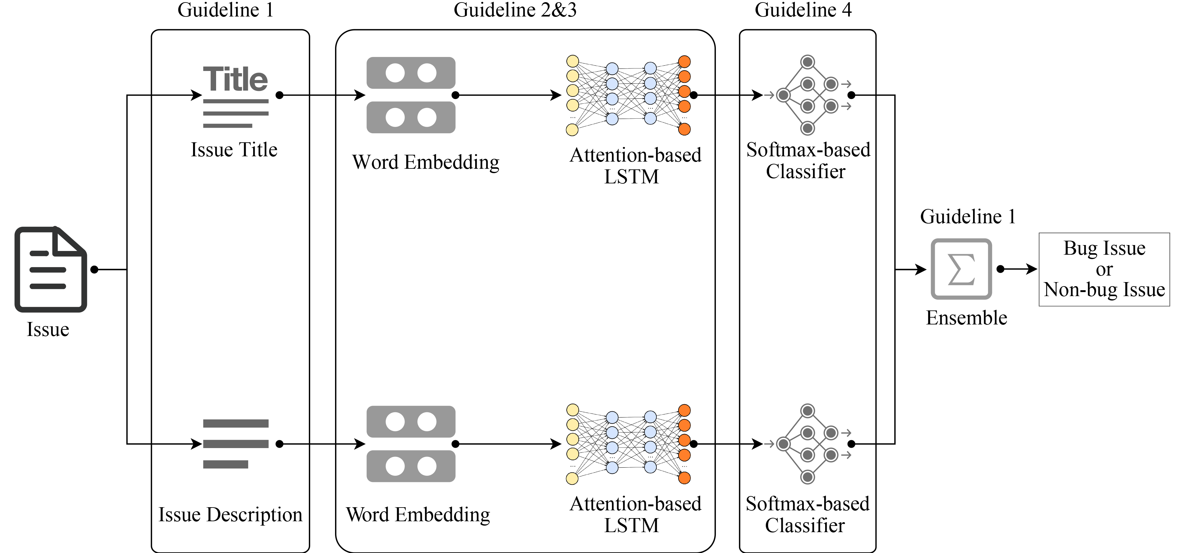
A large body of research effort has been dedicated to automated issue classification for Issue Tracking Systems (ITSs). Although the existing approaches have shown promising performance, the different design choices, including the different textual fields, feature representation methods and machine learning algorithms adopted by existing approaches, have not been comprehensively compared and analyzed. To fill this gap, we perform the first extensive study of automated issue classification on 9 state-of-the-art issue classification approaches. Our experimental results on the widely studied dataset reveal multiple practical guidelines for automated issue classification, including: (1) Training separate models for the issue titles and descriptions and then combining these two models tend to achieve better performance for issue classification; (2) Word embedding with Long Short-Term Memory (LSTM) can better extract features from the textual fields in the issues, and hence, lead to better issue classification models; (3) There exist certain terms in the textual fields that are helpful for building more discriminating classifiers between bug and non-bug issues; (4) The performance of the issue classification model is not sensitive to the choices of ML algorithms. Based on our study outcomes, we further propose an advanced issue classification approach, DEEPLABEL, which can achieve better performance compared with the existing issue classification approaches.
Fig.1 Example of a Jira issue from the HttpClient project with BugID “HttpClient-705”. Names are redacted due to data privacy concerns
Fig.2 The workflow of automatic issue classification
Project
# of issue
# of bugs
# of non-bugs
Jackrabbit
2,402
938
1,464
Lucene
2,443
697
1,746
HttpClient
746
305
441
Total
5,591
1,940
3,651
Tab.1 Detailed information on the dataset HerzigDataset
Approach name
Textual field x
FRM for fext
ML algorithm for fcls
Original dataset
Metrics
Antoniol
Description
TFM
NB,LR,DT
Own Dataset
Precision and recall for each issue type
Chawla
Title
TFM
Fuzzy Logic
HerzigDataset
Precision, recall and F1 score in the granularity of micro-averaging
Pandey
TFM
NB, SVM, LR
Otoom
Reduced TFM
NB,SVM,RF
Own Dataset
Accuracy
Terdchanakul
The concatenation of title and description
n-gram IDF
LR,RF
HerzigDataset
F1 score in the granularity of micro-averaging
Pingclasai
Topic Modeling
DT,NB,LR
Qin
Word Embedding with LSTM
Softmax Layer
Kallis
fastText
fastText
Own Dataset
Precision, recall and F1 score in the granularity of micro-averaging
Herbold
Using separate models for title and description
fastText
fastText
HerzigDataset
Tab.2 Studied Approaches in this study. Column “Textual Field x” lists the textual field x used by each studied approach; Column “FRM for fext” lists the feature representation methods used to construct the feature extractor fext; Column “ML algorithm for fcls” lists the ML algorithms used to build the classifier fcls; Column “Dataset” lists the issue dataset in the paper of the approach, where “Own Dataset” denotes the dataset constructed by the approach itself; Column “Metrics” lists the evaluation metrics used in the paper of the approach
Fig.3
Approach
Bug
Non-Bug
Overall
precision
recall
F1
precision
recall
F1
precision
recall
F1
Chawla
0.73
0.49
0.59
0.77
0.90
0.83
0.76
0.76
0.75
Pandey
0.78
0.70
0.74
0.85
0.89
0.87
0.83
0.83
0.83
Otoom
0.24
0.03
0.05
0.64
0.94
0.76
0.51
0.63
0.52
Terdchanakul
0.58
0.33
0.42
0.71
0.87
0.78
0.67
0.68
0.66
Pingclasai
0.41
0.41
0.41
0.69
0.69
0.69
0.60
0.60
0.60
Qin
0.78
0.75
0.76
0.87
0.87
0.87
0.84
0.84
0.84
Kallis
0.78
0.71
0.74
0.85
0.88
0.87
0.83
0.83
0.83
Herbold
0.82
0.72
0.77
0.86
0.91
0.89
0.85
0.85
0.85
Tab.3 Performance of different Issue Classification Approaches. The Antoniol approach is not listed due to its feature selection can not terminate on HerzigDataset
Approach
Strategy
Bug
Non-Bug
Overall
precision
recall
F1
precision
recall
F1
precision
recall
F1
Chawla
Title
0.73 (AB)
0.49 (A)
0.59 (A)
0.77 (A)
0.90 (B)
0.83 (A)
0.76 (A)
0.76 (A)
0.75 (A)
Desc
0.59 (C)
0.13 (B)
0.22 (B)
0.67 (B)
0.94 (A)
0.78 (B)
0.64 (B)
0.66 (B)
0.59 (B)
Comb1
0.64 (B)
0.14 (B)
0.22 (B)
0.67 (B)
0.95 (A)
0.79 (AB)
0.66 (B)
0.67 (B)
0.59 (B)
Comb2
0.75 (A)
0.50 (A)
0.60 (A)
0.77 (A)
0.91 (B)
0.83 (A)
0.77 (A)
0.77 (A)
0.76 (A)
Pandey
Title
0.78 (A)
0.70 (A)
0.74 (A)
0.85 (A)
0.89 (A)
0.87 (A)
0.83 (A)
0.83 (A)
0.83 (A)
Desc
0.70 (C)
0.63 (B)
0.66 (C)
0.81 (B)
0.85 (B)
0.83 (C)
0.77 (B)
0.78 (B)
0.77 (B)
Comb1
0.74 (B)
0.72 (A)
0.73 (B)
0.85 (A)
0.86 (B)
0.86 (B)
0.81 (AB)
0.81 (AB)
0.81 (AB)
Comb2
0.79 (A)
0.71 (A)
0.75 (A)
0.85 (B)
0.90 (A)
0.87 (A)
0.84 (A)
0.84 (A)
0.84 (A)
Otoom
Title
0.24 (B)
0.03 (?)
0.05 (B)
0.64 (?)
0.94 (?)
0.76 (?)
0.51 (?)
0.63 (?)
0.52 (?)
Desc
0.28 (A)
0.02 (?)
0.05 (B)
0.65 (?)
0.95 (?)
0.77 (?)
0.52 (?)
0.63 (?)
0.52 (?)
Comb1
0.27 (A)
0.05 (?)
0.09 (A)
0.65 (?)
0.92 (?)
0.75 (?)
0.52 (?)
0.62 (?)
0.53 (?)
Comb2
0.25 (B)
0.03 (?)
0.05 (B)
0.65 (?)
0.96 (?)
0.77 (?)
0.52 (?)
0.64 (?)
0.53 (?)
Terdchanakul
Title
0.66 (B)
0.30 (B)
0.41 (?)
0.71 (?)
0.92 (A)
0.80 (A)
0.70 (A)
0.70(B)
0.67 (B)
Desc
0.58 (C)
0.35 (A)
0.43 (?)
0.71 (?)
0.86 (B)
0.78 (B)
0.67 (B)
0.69 (B)
0.66 (B)
Comb1
0.58 (C)
0.33 (A)
0.42 (?)
0.71 (?)
0.87 (B)
0.78 (B)
0.67 (B)
0.68 (B)
0.66 (B)
Comb2
0.69 (A)
0.29 (B)
0.40 (?)
0.71 (?)
0.93 (A)
0.81 (A)
0.71 (A)
0.71 (A)
0.70 (A)
Pingclasai
Title
0.50 (B)
0.12 (B)
0.19 (C)
0.66 (?)
0.93 (A)
0.77 (B)
0.61 (B)
0.65 (B)
0.57 (C)
Desc
0.42 (C)
0.37 (A)
0.39 (A)
0.68 (?)
0.73 (B)
0.70 (C)
0.60 (B)
0.61 (C)
0.60 (B)
Comb1
0.41 (C)
0.41 (A)
0.41 (A)
0.69 (?)
0.69 (B)
0.69 (C)
0.60 (B)
0.60 (C)
0.60 (B)
Comb2
0.66 (A)
0.17 (B)
0.27 (B)
0.68 (?)
0.95 (A)
0.80 (A)
0.68 (A)
0.68 (A)
0.62 (A)
Qin
Ttitle
0.77 (B)
0.72 (B)
0.74 (B)
0.86 (A)
0.88 (B)
0.87 (B)
0.83 (AB)
0.83 (AB)
0.83 (AB)
Desc
0.71 (C)
0.70 (C)
0.70 (C)
0.84 (B)
0.84 (C)
0.84 (C)
0.80 (B)
0.79 (B)
0.79 (B)
Comb1
0.78 (B)
0.75 (A)
0.76 (A)
0.87 (A)
0.87 (B)
0.87 (B)
0.84 (A)
0.84 (A)
0.84 (A)
Comb2
0.82 (A)
0.74 (A)
0.77 (A)
0.87 (A)
0.90 (A)
0.89 (A)
0.85 (A)
0.85 (A)
0.85 (A)
Kallis
Title
0.77 (B)
0.72 (A)
0.74 (B)
0.86 (A)
0.88 (B)
0.87 (B)
0.83 (B)
0.83 (B)
0.83 (B)
Desc
0.74 (C)
0.62 (B)
0.67 (C)
0.81 (B)
0.88 (B)
0.84 (C)
0.79 (C)
0.79 (C)
0.79 (C)
Comb1
0.78 (B)
0.71 (A)
0.74 (B)
0.85 (A)
0.88 (B)
0.87 (B)
0.83 (B)
0.83 (B)
0.83 (B)
Comb2
0.82 (A)
0.72 (A)
0.77 (A)
0.86 (A)
0.91 (A)
0.89 (A)
0.85 (A)
0.85 (A)
0.85 (A)
Tab.4 Comparing different types of classifiers. The four types of classifiers for the Herbold approach are the same as the four types of classifiers for the Kallis approach and hence elided. The capital letters A-C in the parentheses are the results of the Tukey HSD test, where techniques are clustered into the letter groups, and A is the best while C is the worst (and having two letters means the technique is in a group that is between the two letter groups). Symbol “?” denotes the Tukey HSD test fails to observe a statistical difference between the four strategies
Fig.4 The detailed analysis of results on trategy Title and Strategy Desc. (a) The ratio of the number of issues that are classified differently by Strategy Title and Strategy Desc to the number of testing issues. (b) The ratio of the number of issues that are correctly predicted by Strategy Title (or Desc) to the number of issues that are classified differently by the two classifier types
Fig.5
Fig.6
Fig.7
Classifier
FRM
Bug
Non-Bug
Overall
precision
recall
F1
precision
recall
F1
precision
recall
F1
LR
word embedding with LSTM
0.82 (A)
0.74 (A)
0.78 (A)
0.87 (A)
0.91 (B)
0.89 (A)
0.85 (A)
0.85 (A)
0.85 (A)
fastText
0.73 (C)
0.38 (B)
0.50 (B)
0.74 (B)
0.93 (B)
0.82 (B)
0.74 (B)
0.74 (B)
0.71 (B)
TFM
0.80 (B)
0.72 (A)
0.76 (A)
0.86 (A)
0.90 (C)
0.88 (A)
0.84 (A)
0.84 (A)
0.84 (A)
reduced TFM
0.00 (E)
0.00 (E)
0.00 (E)
0.65 (C)
1.00 (A)
0.79 (C)
0.43 (D)
0.65 (C)
0.52 (D)
topic modeling
0.66 (D)
0.17 (D)
0.27 (D)
0.68 (BC)
0.94 (B)
0.79 (C)
0.68 (C)
0.68 (C)
0.61 (C)
n-gram IDF
0.72 (C)
0.25 (C)
0.37 (C)
0.70 (BC)
0.94 (B)
0.80 (B)
0.71 (BC)
0.70 (BC)
0.66 (BC)
RF
word embedding with LSTM
0.81 (A)
0.74 (A)
0.78 (A)
0.87 (A)
0.91 (C)
0.89 (A)
0.85 (A)
0.85 (A)
0.85 (A)
fastText
0.80 (A)
0.18 (D)
0.30 (D)
0.69 (D)
0.97 (B)
0.80 (B)
0.73 (C)
0.70 (CD)
0.63 (D)
TFM
0.81 (A)
0.65 (B)
0.72 (B)
0.83 (B)
0.92 (C)
0.87 (A)
0.83 (B)
0.83 (B)
0.82 (B)
reduced TFM
0.28 (C)
0.00 (E)
0.00 (E)
0.65 (E)
0.99 (A)
0.78 (C)
0.54 (E)
0.65 (D)
0.51 (E)
topic modeling
0.49 (C)
0.23 (C)
0.32 (D)
0.68 (D)
0.87 (D)
0.76 (D)
0.62 (D)
0.65 (D)
0.61 (D)
n-gram IDF
0.69 (B)
0.28 (C)
0.40 (C)
0.71 (C)
0.93 (C)
0.80 (B)
0.70 (C)
0.71 (C)
0.67 (C)
DT
word embedding with LSTM
0.65 (A)
0.86 (A)
0.74 (A)
0.91 (A)
0.75 (C)
0.82 (A)
0.82 (A)
0.79 (A)
0.79 (A)
fastText
0.41 (C)
0.66 (B)
0.50 (C)
0.73 (C)
0.49 (E)
0.59 (D)
0.62 (D)
0.55 (D)
0.56 (E)
TFM
0.57 (B)
0.84 (A)
0.68 (B)
0.88 (B)
0.67 (D)
0.76 (B)
0.78 (B)
0.73 (B)
0.73 (B)
reduced TFM
0.29 (D)
0.00 (E)
0.01 (E)
0.65 (D)
0.99 (A)
0.78 (AB)
0.53 (E)
0.64 (C)
0.51 (F)
topic modeling
0.41 (C)
0.40 (C)
0.40 (D)
0.68 (CD)
0.69 (D)
0.68 (C)
0.59 (DE)
0.59 (D)
0.59 (D)
n-gram IDF
0.68 (A)
0.28 (D)
0.39 (D)
0.71 (CD)
0.92 (B)
0.80 (AB)
0.70 (C)
0.70 (B)
0.66 (C)
Softmax
word embedding with LSTM
0.81 (A)
0.73 (B)
0.77 (A)
0.86 (A)
0.90 (B)
0.88 (A)
0.85 (A)
0.85 (A)
0.85 (A)
fastText
0.33 (D)
0.94 (A)
0.49 (C)
0.32 (E)
0.01 (C)
0.02 (C)
0.33 (F)
0.33 (D)
0.18 (E)
TFM
0.80 (A)
0.64 (C)
0.71 (B)
0.82 (B)
0.91 (B)
0.87 (A)
0.82 (B)
0.82 (B)
0.81 (B)
reduced TFM
0.00 (E)
0.00 (E)
0.00 (E)
0.65 (D)
1.00 (A)
0.78 (B)
0.42 (E)
0.65 (C)
0.51 (D)
topic modeling
0.52 (C)
0.03 (E)
0.07 (E)
0.65 (D)
0.98 (A)
0.78 (B)
0.62 (D)
0.66 (C)
0.54 (D)
n-gram IDF
0.74 (B)
0.09 (D)
0.16 (D)
0.67 (C)
0.97 (AB)
0.79 (AB)
0.70 (C)
0.67 (C)
0.58 (C)
Tab.5 Comparing different feature representation methods. The capital letters A-F in the parentheses are the results of the Tukey HSD test, where techniques are clustered into the letter groups, and A is the best while F is the worst (and having two letters means the technique is in a group that is between the two letter groups). Symbol “?” denotes the Tukey HSD test fails to observe a statistical difference between the six feature representation methods
Fig.8
Fig.9
FRM
Classifier
Bug
Non-Bug
Overall
precision
recall
F1
precision
recall
F1
precision
recall
F1
word embedding with LSTM
LR
0.82 (A)
0.74 (B)
0.78 (A)
0.87 (B)
0.91 (A)
0.89 (A)
0.85 (A)
0.85 (A)
0.85 (A)
RF
0.81 (A)
0.74 (B)
0.78 (A)
0.87 (B)
0.91 (A)
0.89 (A)
0.85 (AB)
0.85 (A)
0.85 (A)
DT
0.65 (B)
0.86 (A)
0.74 (B)
0.91 (A)
0.75 (B)
0.82 (B)
0.82 (B)
0.79 (B)
0.79 (B)
Softmax
0.81 (A)
0.73 (B)
0.77 (AB)
0.86 (B)
0.90 (A)
0.88 (A)
0.85 (AB)
0.85 (A)
0.85 (A)
fastText
LR
0.73 (B)
0.38 (C)
0.50 (A)
0.74 (A)
0.93 (B)
0.82 (A)
0.74 (A)
0.74 (A)
0.71 (A)
RF
0.80 (A)
0.18 (D)
0.30 (B)
0.69 (A)
0.97 (A)
0.80 (B)
0.73 (B)
0.70 (A)
0.63 (B)
DT
0.41 (C)
0.66 (B)
0.50 (A)
0.73 (A)
0.49 (C)
0.59 (C)
0.62 (C)
0.55 (B)
0.56 (C)
Softmax
0.33 (C)
0.94 (A)
0.49 (A)
0.32 (B)
0.01 (D)
0.02 (D)
0.33 (D)
0.33 (C)
0.18 (D)
TFM
LR
0.80 (A)
0.72 (B)
0.76 (A)
0.86 (B)
0.90 (A)
0.88 (A)
0.84 (A)
0.84 (A)
0.84 (A)
RF
0.81 (A)
0.65 (C)
0.72 (AB)
0.83 (B)
0.92 (A)
0.87 (A)
0.83 (A)
0.83 (A)
0.82 (A)
DT
0.57 (B)
0.84 (A)
0.68 (B)
0.88 (A)
0.67 (B)
0.76 (B)
0.78 (B)
0.73 (B)
0.73 (B)
Softmax
0.80 (A)
0.64 (C)
0.71 (AB)
0.82 (B)
0.91 (A)
0.87 (A)
0.82 (AB)
0.82 (A)
0.81 (A)
reduced TFM
LR
0.00 (B)
0.00 (B)
0.00 (B)
0.65 (?)
1.00 (A)
0.79 (?)
0.43 (B)
0.65 (?)
0.52 (?)
RF
0.28 (A)
0.00 (AB)
0.00 (AB)
0.65 (?)
0.99 (B)
0.78 (?)
0.54 (A)
0.65 (?)
0.51 (?)
DT
0.29 (A)
0.00 (A)
0.01 (A)
0.65 (?)
0.99 (C)
0.78 (?)
0.53 (A)
0.64 (?)
0.51 (?)
Softmax
0.00 (B)
0.00 (B)
0.00 (B)
0.65 (?)
1.00 (AB)
0.78 (?)
0.42 (B)
0.65 (?)
0.51 (?)
topic modeling
LR
0.66 (A)
0.17 (C)
0.27 (B)
0.68 (?)
0.94 (B)
0.79 (A)
0.68 (A)
0.68 (A)
0.61 (A)
RF
0.49 (B)
0.23 (B)
0.32 (B)
0.68 (?)
0.87 (C)
0.76 (A)
0.62 (B)
0.65 (A)
0.61 (A)
DT
0.41 (B)
0.40 (A)
0.40 (A)
0.68 (?)
0.69 (D)
0.68 (B)
0.59 (B)
0.59 (B)
0.59 (AB)
Softmax
0.52 (AB)
0.03 (D)
0.07 (C)
0.65 (?)
0.98 (A)
0.78 (A)
0.62 (B)
0.66 (A)
0.54 (B)
n-gram IDF
LR
0.72 (?)
0.25 (A)
0.37 (A)
0.70 (?)
0.94 (B)
0.80 (?)
0.71 (?)
0.70 (?)
0.66 (A)
RF
0.69 (?)
0.28 (A)
0.40 (A)
0.71 (?)
0.93 (B)
0.80 (?)
0.70 (?)
0.71 (?)
0.67 (A)
DT
0.68 (?)
0.28 (A)
0.39 (A)
0.71 (?)
0.92 (B)
0.80 (?)
0.70 (?)
0.70 (?)
0.66 (A)
Softmax
0.74 (?)
0.09 (B)
0.16 (B)
0.67 (?)
0.97 (A)
0.79 (?)
0.70 (?)
0.67 (?)
0.58 (B)
Tab.6 Comparing different machine learning algorithms. The capital letters A-D in the parentheses are the results of the Tukey HSD test, where techniques are clustered into the letter groups, and A is the best while D is the worst (and having two letters means the technique is in a group that is between the two letter groups). Symbol “?” denotes the Tukey HSD test fails to observe a statistical difference between the four machine learning algorithms
Fig.10
Fig.11 The overview of DEEPLABEL
Approach
Merformance metrics
Statistical testing
Bug
Non-Bug
Overall
Bug
Non-Bug
Overall
precision
recall
F1
precision
recall
F1
precision
recall
F1
precision
recall
F1
precision
recall
F1
precision
recall
F1
Chawla
0.73
0.49
0.59
0.77
0.90
0.83
0.76
0.76
0.75
0.86
0.86
1.00
0.97
0.21
0.84
0.94
0.93
0.97
Pandey
0.78
0.70
0.74
0.85
0.89
0.87
0.83
0.83
0.83
0.49
0.54
0.67
0.58
0.30
0.40
0.69
0.65
0.67
Otoom
0.24
0.03
0.05
0.64
0.94
0.76
0.51
0.63
0.52
1.00
1.00
1.00
?0.64
1.00
0.94
1.00
1.00
1.00
Terdchanakul
0.58
0.33
0.42
0.71
0.87
0.78
0.67
0.68
0.66
1.00
1.00
1.00
1.00
1.00
1.00
1.00
1.00
1.00
Pingclasai
0.41
0.41
0.41
0.69
0.69
0.69
0.60
0.60
0.60
1.00
1.00
1.00
1.00
1.00
1.00
1.00
1.00
1.00
Qin
0.78
0.75
0.76
0.87
0.87
0.87
0.84
0.84
0.84
0.65
0.09
0.50
0.18
0.35
0.28
0.44
0.43
0.42
Kallis
0.78
0.71
0.74
0.85
0.88
0.87
0.83
0.83
0.83
0.48
0.44
0.68
0.50
0.26
0.40
0.63
0.58
0.60
Herbold
0.82
0.72
0.77
0.86
0.91
0.89
0.85
0.85
0.85
0.00
0.47
0.38
0.38
?0.05
0.16
0.30
0.29
0.30
BERT-Title
0.77
0.78
0.77
0.88
0.87
0.87
0.84
0.84
0.84
0.62
?0.20
0.28
0.02
0.48
0.30
0.32
0.38
0.31
BERT-Desc
0.72
0.70
0.71
0.84
0.85
0.84
0.80
0.80
0.80
0.88
0.56
0.90
0.66
0.66
0.70
0.82
0.82
0.82
BERT-Comb1
0.78
0.79
0.78
0.89
0.88
0.88
0.85
0.85
0.85
0.42
?0.34
0.16
?0.10
0.42
0.16
0.16
0.19
0.15
DEEPLABEL
0.82
0.77
0.79
0.88
0.91
0.89
0.86
0.86
0.86
?
Tab.7 Effectiveness comparison between DEEPLABEL and the previous techniques on HerzigDataset. Colum “Statistical Testing” presents the values of the Cliff’s delta effect size between HerzigDataset and each of the compared approaches. We highlight the statistical results using , and , when the Wilcoxon signed-rank test satisfy p<0.001, p<0.01, p<0.05, respectively. Symbol “?” means not available in those cases
Fig.12
ITS
# of issue
# of porjects
# of bugs
Jira
Apache
879,602
620
467,069
JBoss
354,852
418
172,104
Spring
66,404
95
26,163
GitHub
184,834
50
75,277
Total
1,485,693
1,183
740,613
Tab.8 Detailed information on the dataset LargeDataset
Approach
Performance metrics
Statistical testing
Bug
Non-Bug
Overall
Bug
Non-Bug
Overall
precision
recall
F1
precision
recall
F1
precision
recall
F1
precision
recall
F1
precision
recall
F1
precision
recall
F1
Chawla
0.79
0.61
0.67
0.69
0.82
0.72
0.75
0.70
0.69
0.36
0.80
1.00
0.80
?0.70
0.80
1.00
1.00
1.00
Pandey
0.80
0.74
0.77
0.75
0.82
0.78
0.78
0.78
0.78
0.68
1.00
1.00
0.80
?0.24
0.62
1.00
1.00
1.00
Otoom
0.56
0.90
0.69
0.76
0.29
0.42
0.66
0.59
0.55
1.00
?0.88
1.00
0.8
1.00
1.00
1.00
1.00
1.00
Terdchanakul
0.67
0.61
0.63
0.64
0.70
0.66
0.67
0.65
0.65
1.00
1.00
1.00
1.00
0.84
1.00
1.00
1.00
1.00
Pingclasai
0.71
0.68
0.69
0.67
0.71
0.69
0.70
0.69
0.69
1.00
1.00
1.00
0.96
0.90
1.00
1.00
1.00
1.00
Qin
0.82
0.84
0.83
0.83
0.82
0.82
0.82
0.82
0.82
0.17
0.28
0.43
?0.12
?0.25
?0.17
0.26
0.23
0.24
Kallis
0.79
0.82
0.80
0.81
0.78
0.80
0.80
0.80
0.80
0.78
0.56
0.78
0.29
0.42
0.39
0.76
0.80
0.80
Herbold
0.81
0.84
0.82
0.82
0.79
0.80
0.81
0.81
0.81
0.48
0.34
0.52
0.27
0.44
0.43
0.58
0.62
0.60
BERT-Title
0.81
0.83
0.82
0.83
0.82
0.82
0.82
0.82
0.82
0.43
0.46
0.62
0.07
0.13
0.05
0.49
0.48
0.48
BERT-Desc
0.79
0.83
0.80
0.80
0.77
0.78
0.80
0.80
0.80
0.76
0.50
0.70
0.48
0.68
0.64
0.94
0.94
0.94
BERT-Comb1
0.82
0.85
0.84
0.84
0.83
0.84
0.83
0.83
0.83
0.2
0.18
0.34
?0.27
?0.44
?0.20
0.32
0.32
0.32
DEEPLABEL
0.85
0.86
0.86
0.83
0.82
0.83
0.85
0.85
0.85
?
Tab.9 Effectiveness comparison between DEEPLABEL and the previous techniques on LargeDataset. Colum “Statistical Testing” presents the values of the Cliff’s delta effect size between DEEPLABEL and each of the compared approaches. We highlight the statistical results using , and , when the Wilcoxon signed-rank test satisfy p<0.001, p<0.01, p<0.05, respectively. Symbol “?” means not available in those cases
Fig.13
Approach
Overall performance
Statistical testing
precision
recall
F1
precision
recall
F1
Pandey
0.66
0.64
0.63
?0.16
0.18
0.19
Terdchanakul
0.31
0.38
0.27
1.00
1.00
1.00
Pingclasai
0.35
0.39
0.34
1.00
1.00
1.00
Qin
0.37
0.39
0.31
1.00
1.00
1.00
Kallis
0.48
0.56
0.48
1.00
0.98
1.00
Herbold
0.63
0.65
0.62
0.24
0.16
0.46
DEEPLABEL
0.65
0.66
0.65
?
Tab.10 Effectiveness comparison between DEEPLABEL and the previous techniques on multi-classification problem. The Chawla approach and the Otoom approach are not included in the table because they are not available for multi-classification problems. Colum “Statistical Testing” presents the values of the Cliff’s delta effect size between DEEPLABEL and each of the compared approaches. We highlight the statistical results using , and , when the Wilcoxon signed-rank test satisfy p<0.001, p<0.01, p<0.05, respectively. Symbol “?” means not available in those cases
Field
Keywords
Title
support, should, add, error, not, doesnt, fail, fix, update, remove, improve, wrong, upgrade, need, miss
Description
support, current, add, fail, need, should, not, codeseg, would, hyperlink, improve, remove, fix, error, provide
Tab.11 The words on which the attention mechanism applies the largest attention weights when detecting bug issues. The first row presents the words from the issue titles, and the second row presents the words from the issue descriptions
1
T, Merten B, Mager P, Hübner T, Quirchmayr B, Paech S Bürsner . Requirements communication in issue tracking systems in four open-source projects. In: Proceedings of the Joint Proceedings of REFSQ-2015 Workshops, Research Method Track, and Poster Track Co-Located with the 21st International Conference on Requirements Engineering: Foundation for Software Quality. 2015, 114−125
2
D, Bertram A, Voida S, Greenberg R Walker . Communication, collaboration, and bugs: the social nature of issue tracking in small, collocated teams. In: Proceedings of 2010 ACM Conference on Computer Supported Cooperative Work. 2010, 291−300
3
T F, Bissyandé D, Lo L, Jiang L, Réveillère J, Klein Traon Y Le . Got issues? Who cares about it? A large scale investigation of issue trackers from GitHuB. In: Proceedings of the 24th International Symposium on Software Reliability Engineering. 2013, 188−197
4
Y, Yan D, Cheng J E, Feng H, Li J Yue . Survey on applications of algebraic state space theory of logical systems to finite state machines. Science China Information Sciences, 2023, 66( 1): 111201
5
Q, Fan Y, Yu G, Yin T, Wang H Wang . Where is the road for issue reports classification based on text mining?. In: Proceedings of 2017 ACM/IEEE International Symposium on Empirical Software Engineering and Measurement. 2017, 121−130
6
S, Breu R, Premraj J, Sillito T Zimmermann . Information needs in bug reports: improving cooperation between developers and users. In: Proceedings of 2010 ACM Conference on Computer Supported Cooperative Work. 2010, 301−310
7
N, Limsettho H, Hata A, Monden K Matsumoto . Automatic unsupervised bug report categorization. In: Proceedings of the 6th International Workshop on Empirical Software Engineering in Practice. 2014, 7−12
8
M, Hammad R, Alzyoudi A F Otoom . Automatic clustering of bug reports. International Journal of Advanced Computer Research, 2018, 8( 39): 313–323
9
I, Chawla S K Singh . Automated labeling of issue reports using semi supervised approach. Journal of Computational Methods in Sciences and Engineering, 2018, 18( 1): 177–191
10
G, Antoniol K, Ayari Penta M, Di F, Khomh Y G Guéhéneuc . Is it a bug or an enhancement?: a text-based approach to classify change requests. In: Proceedings of the 28th Annual International Conference on Computer Science and Software Engineering. 2018, 2−16
11
N, Pingclasai H, Hata K I Matsumoto . Classifying bug reports to bugs and other requests using topic modeling. In: Proceedings of the 20th Asia-Pacific Software Engineering Conference. 2013, 13−18
12
N, Limsettho H, Hata K I Matsumoto . Comparing hierarchical dirichlet process with latent dirichlet allocation in bug report multiclass classification. In: Proceedings of the 15th IEEE/ACIS International Conference on Software Engineering, Artificial Intelligence, Networking and Parallel/Distributed Computing. 2014, 1−6
13
I, Chawla S K Singh . An automated approach for bug categorization using fuzzy logic. In: Proceedings of the 8th India Software Engineering Conference. 2015, 90−99
14
Y, Zhou Y, Tong R, Gu H Gall . Combining text mining and data mining for bug report classification. Journal of Software: Evolution and Process, 2016, 28( 3): 150–176
15
P, Terdchanakul H, Hata P, Phannachitta K Matsumoto . Bug or not? Bug report classification using N-Gram IDF. In: Proceedings of 2017 IEEE International Conference on Software Maintenance and Evolution. 2017, 534−538
16
N, Pandey D K, Sanyal A, Hudait A Sen . Automated classification of software issue reports using machine learning techniques: an empirical study. Innovations in Systems and Software Engineering, 2017, 13( 4): 279–297
17
H, Qin X Sun . Classifying bug reports into bugs and non-bugs using LSTM. In: Proceedings of the 10th Asia-Pacific Symposium on Internetware. 2018, 20
18
M S, Zolkeply J Shao . Classifying software issue reports through association mining. In: Proceedings of the 34th ACM/SIGAPP Symposium on Applied Computing. 2019, 1860−1863
19
A F, Otoom S, Al-Jdaeh M Hammad . Automated classification of software bug reports. In: Proceedings of the 9th International Conference on Information Communication and Management. 2019, 17−21
20
R, Kallis Sorbo A, Di G, Canfora S Panichella . Ticket tagger: machine learning driven issue classification. In: Proceedings of 2019 IEEE International Conference on Software Maintenance and Evolution. 2019, 406−409
21
K, Herzig S, Just A Zeller . It’s not a bug, it’s a feature: how misclassification impacts bug prediction. In: Proceedings of the 35th International Conference on Software Engineering. 2013, 392−401
22
Z, Li M, Pan Y, Pei T, Zhang L, Wang X Li . DeepLabel: automated issue classification for issue tracking systems. In: Proceedings of the 13th Asia-Pacific Symposium on Internetware. 2022, 231−241
23
M, Ortu G, Destefanis M, Kassab M Marchesi . Measuring and understanding the effectiveness of JIRA developers communities. In: Proceedings of the 6th IEEE/ACM International Workshop on Emerging Trends in Software Metrics. 2015, 3−10
24
C Wohlin . Guidelines for snowballing in systematic literature studies and a replication in software engineering. In: Proceedings of the 18th International Conference on Evaluation and Assessment in Software Engineering. 2014, 38
25
N, Limsettho H, Hata A, Monden K Matsumoto . Unsupervised bug report categorization using clustering and labeling algorithm. International Journal of Software Engineering and Knowledge Engineering, 2016, 26( 7): 1027–1053
26
N, Pandey A, Hudait D K, Sanyal A Sen . Automated classification of issue reports from a software issue tracker. In: Sa P K, Sahoo M N, Murugappan M, Wu Y, Majhi B, eds. Progress in Intelligent Computing Techniques: Theory, Practice, and Applications. Singapore: Springer, 2018, 423−430
A, Joulin E, Grave P, Bojanowski T Mikolov . Bag of tricks for efficient text classification. In: Proceedings of the 15th Conference of the European Chapter of the Association for Computational Linguistics. 2017, 427−431
29
S, Herbold A, Trautsch F Trautsch . On the feasibility of automated prediction of bug and non-bug issues. In: Koziolek A, Schaefer I, Seidl C, eds. Software Engineering 2021. Bonn: Gesellschaft für Informatik e.V., 2021, 55−56
30
Q, Perez P A, Jean C, Urtado S Vauttier . Bug or not bug? That is the question. In: Proceedings of the 29th IEEE/ACM International Conference on Program Comprehension. 2021, 47−58
31
A, Trautsch F, Trautsch S, Herbold B, Ledel J Grabowski . The SmartSHARK ecosystem for software repository mining. In: Proceedings of the 42nd International Conference on Software Engineering. 2020, 25−28
32
J, Han M, Kamber J Pei . Data Mining: Concepts and Techniques. 3rd ed. San Francisco: Morgan Kaufmann, 2011
33
P S, Kochhar F, Thung D Lo . Automatic fine-grained issue report reclassification. In: Proceedings of the 19th International Conference on Engineering of Complex Computer Systems. 2014, 126−135
34
Z, Li Y, Yu G, Yin T, Wang Q, Fan H Wang . Automatic classification of review comments in pull-based development model. In: Proceedings of the 29th International Conference on Software Engineering and Knowledge Engineering. 2017, 572−577
35
J W Tukey . Comparing individual means in the analysis of variance. Biometrics, 1949, 5( 2): 99–114
36
A, Vaswani N, Shazeer N, Parmar J, Uszkoreit L, Jones A N, Gomez L, Kaiser I Polosukhin . Attention is all you need. In: Proceedings of the 31st International Conference on Neural Information Processing Systems. 2017, 6000−6010
37
T, Mikolov K, Chen G, Corrado J Dean . Efficient estimation of word representations in vector space. In: Proceedings of the 1st International Conference on Learning Representations. 2013
38
D, Bahdanau K, Cho Y Bengio . Neural machine translation by jointly learning to align and translate. In: Proceedings of the 3rd International Conference on Learning Representations. 2015
39
F Wilcoxon . Individual comparisons by ranking methods. In: Kotz S, Johnson N L, eds. Breakthroughs in Statistics: Methodology and Distribution. New York: Springer, 1992, 196−202
40
N Cliff . Ordinal Methods for Behavioral Data Analysis. New York: Psychology Press, 1996
41
Y, Fan X, Xia Costa D A, da D, Lo A E, Hassan S Li . The impact of mislabeled changes by SZZ on just-in-time defect prediction. IEEE Transactions on Software Engineering, 2021, 47( 8): 1559–1586
42
T, Wolf L, Debut V, Sanh J, Chaumond C, Delangue A, Moi P, Cistac T, Rault R, Louf M, Funtowicz J, Davison S, Shleifer Platen P, von C, Ma Y, Jernite J, Plu C, Xu Scao T, Le S, Gugger M, Drame Q, Lhoest A Rush . Transformers: state-of-the-art natural language processing. In: Proceedings of 2020 Conference on Empirical Methods in Natural Language Processing: System Demonstrations. 2020, 38−45
43
S, Wiegreffe Y Pinter . Attention is not not explanation. In: Proceedings of the 2019 Conference on Empirical Methods in Natural Language Processing and the 9th International Joint Conference on Natural Language Processing. 2019, 11−20
44
C H, Chang E, Creager A, Goldenberg D Duvenaud . Explaining image classifiers by counterfactual generation. In: Proceedings of the 7th International Conference on Learning Representations. 2019
45
P, Dabkowski Y Gal . Real time image saliency for black box classifiers. In: Proceedings of the 31st International Conference on Neural Information Processing Systems. 2017, 6970−6979
46
R, Fong M, Patrick A Vedaldi . Understanding deep networks via extremal perturbations and smooth masks. In: Proceedings of 2019 IEEE/CVF International Conference on Computer Vision. 2019, 2950−2958
47
R C, Fong A Vedaldi . Interpretable explanations of black boxes by meaningful perturbation. In: Proceedings of the IEEE International Conference on Computer Vision. 2017, 3449−3457
48
R R, Selvaraju M, Cogswell A, Das R, Vedantam D, Parikh D Batra . Grad-CAM: visual explanations from deep networks via gradient-based localization. In: Proceedings of the IEEE International Conference on Computer Vision. 2017, 618−626
49
A, Shrikumar P, Greenside A Kundaje . Learning important features through propagating activation differences. In: Proceedings of the 34th International Conference on Machine Learning. 2017, 3145−3153
50
J T, Springenberg A, Dosovitskiy T, Brox M A Riedmiller . Striving for simplicity: the all convolutional net. In: Proceedings of the 3rd International Conference on Learning Representations. 2015
51
M T, Ribeiro S, Singh C Guestrin . "Why should I trust you?": explaining the predictions of any classifier. In: Proceedings of the 22nd ACM SIGKDD International Conference on Knowledge Discovery and Data Mining. 2016, 1135−1144
52
S M, Lundberg S I Lee . A unified approach to interpreting model predictions. In: Proceedings of the 31st International Conference on Neural Information Processing Systems. 2017, 4768−4777
53
W, Guo D, Mu J, Xu P, Su G, Wang X Xing . LEMNA: explaining deep learning based security applications. In: Proceedings of 2018 ACM SIGSAC Conference on Computer and Communications Security. 2018, 364−379
54
M, Gegick P, Rotella T Xie . Identifying security bug reports via text mining: an industrial case study. In: Proceedings of the 7th International Working Conference on Mining Software Repositories. 2010, 11−20
55
H B, McMahan G, Holt D, Sculley M, Young D, Ebner J, Grady L, Nie T, Phillips E, Davydov D, Golovin S, Chikkerur D, Liu M, Wattenberg A M, Hrafnkelsson T, Boulos J Kubica . Ad click prediction: a view from the trenches. In: Proceedings of the 19th ACM SIGKDD International Conference on Knowledge Discovery and Data Mining. 2013, 1222−1230
56
D, Sahoo Q, Pham J, Lu S C H Hoi . Online deep learning: learning deep neural networks on the fly. In: Proceedings of the 27th International Joint Conference on Artificial Intelligence. 2018, 2660−2666
57
S C H, Hoi D, Sahoo J, Lu P Zhao . Online learning: a comprehensive survey. Neurocomputing, 2021, 459: 249–289