Development of the DayCent-Photo model and integration of variable photosynthetic capacity

doi:10.1007/s11707-018-0736-6

Front. Earth Sci.

2018, Vol. 12

Issue (4) : 765-778 https://doi.org/10.1007/s11707-018-0736-6

RESEARCH ARTICLE

Development of the DayCent-Photo model and integration of variable photosynthetic capacity

Jonathan R. STRAUBE^1,²(

), Maosi CHEN¹, William J. PARTON^1,², Shinichi ASSO^1,², Yan-An LIU^3,^4,^5,¹(

), Dennis S. OJIMA², Wei GAO^1,^6,⁵

¹. USDA UV-B Monitoring and Research Program, Natural Resource Ecology Laboratory, Colorado State University, Fort Collins, CO 80521, USA
². Natural Resource Ecology Laboratory, Colorado State University, Fort Collins, CO 80523, USA
³. Key Laboratory of Geographic Information Science (Ministry of Education), East China Normal University, Shanghai 200241, China
⁴. School of Geographic Sciences, East China Normal University, Shanghai 200241, China
⁵. ECNU-CSU Joint Research Institute for New Energy and the Environment, Shanghai 200062, China
⁶. Department of Ecosystem Science and Sustainability, Colorado State University, Fort Collins, CO 80523, USA

Download: PDF(1971 KB) HTML
Export: BibTeX | EndNote | Reference Manager | ProCite | RefWorks

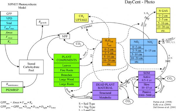
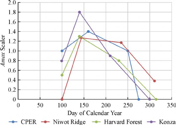
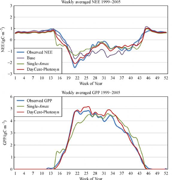
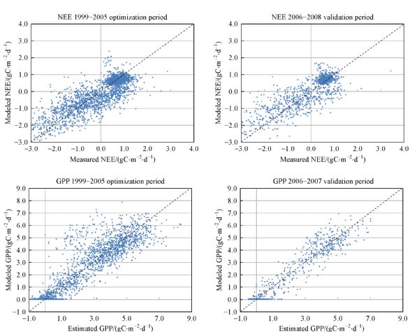
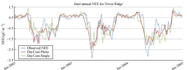
Abstract

We integrated a photosynthetic sub-model into the daily Century model (DayCent) to improve the estimations of seasonal changes in carbon fluxes at the Niwot Ridge LTER site and the Harvard forest LTER site (DayCent-Photo). The photosynthetic sub-model, adapted from the SIPNET/PnET family of models, includes solar radiation and vapor pressure deficit controls on production, as well as temperature and water stress terms. A key feature we added to the base photosynthetic equations is the addition of a variable maximum net photosynthetic rate (Amax). We optimized the parameters controlling photosynthesis using a variation of the Metropolis-Hastings algorithm along with data-assimilation techniques. The model was optimized and validated against observed net ecosystem exchange (NEE) and estimated gross primary production (GPP) and ecosystem respiration (RESP) values for AmeriFlux sites at Niwot Ridge and Harvard forest. The inclusion of a variable Amax rate greatly improved model performance (NEE RMSE= 0.63 gC·m⁻², AIC= 2099) versus a version with a single Amax parameter (NEE RMSE= 0.74 gC·m⁻², AIC= 3724). DayCent-Photo was able to capture the inter-annual and seasonal flux patterns for NEE, GPP, ecosystem respiration (RESP), and daily actual evapotranspiration (AET), but tended to overestimate yearly NEE uptake. The DayCent-Photo model has been successfully set up to simulate daily NEE, GPP, RESP, and AET for deciduous forest, conifer forests, and grassland systems in the US using AmeriFlux data sets and has recently been improved to include the impact of UV radiation surface litter decay (DayCent-UV). The simulated influence of a variable Amax rate suggests a need for further studies on the process controls affecting the seasonal photosynthetic rates. The results for all of the forest and grassland sites show that maximum Amax values occurs early during the growing period and taper off toward the end of the growing season.

Keywords DayCent-Photo model seasonal maximum net photosynthetic rate net ecosystem exchange gross primary production UV radiation

Corresponding Author(s): Jonathan R. STRAUBE,Yan-An LIU

Just Accepted Date: 12 September 2018 Online First Date: 26 October 2018 Issue Date: 20 November 2018

Cite this article:

Jonathan R. STRAUBE,Maosi CHEN,William J. PARTON, et al. Development of the DayCent-Photo model and integration of variable photosynthetic capacity[J]. Front. Earth Sci., 2018, 12(4): 765-778.

URL:

https://academic.hep.com.cn/fesci/EN/10.1007/s11707-018-0736-6
https://academic.hep.com.cn/fesci/EN/Y2018/V12/I4/765

Fig.1 The DayCent model with the photosynthetic modifications. Maintenance respiration is based on the PS2Mrsp parameter.

Fig.2 The optimized seasonal values of Amax at Niwot Ridge, CPER, Harvard Forest, and Konza sites.

Tab.1 Photosynthetic parameters, starting values and ranges. Parameters marked with an (*) are taken from ^{Moore et al. (2008)}. Values marked with a (#) are from Sarah Davis, personal communication. Estimates for PS2Mrsp are taken from literature values for maintenance respiration (Ryan and Waring, 1992). Fixed parameters do not change during the optimization process. Parameters are considered to have no units unless labeled otherwise

Tab.2 Parameters marked with (#) are fixed and do not vary during optimization. The numbers beside the best parameter set are parameterizations from the runs that were statistically similar (P = 0.05) in terms of likelihood. With the first number being the mean and the number after (±) being the standard deviation of the mean

Tab.3 Model comparison for DayCent model. Single-Amax is the photosynthetic version of DayCent with a single Amax value. DayCent-Photo is the photosynthetic model with seasonal variation of Amax. Root Mean Square Error (RMSE) is a measure of the amount of variance not explained by the model, lower is better. Akaike Information Criterion (AIC) equation is 2K– 2ln(L), where ln(L) = Ltotal. A lower AIC indicates the model that has better support from the data

Fig.3 Model comparison of GPP and NEE for the optimization period from 1999?2005. The data is averaged into 52 weekly periods. Note there is no GPP data for the Base DayCent model because the Base DayCent model where DayCent-Photo is developed from does not have the specialized module for GPP calculation.

Fig.4 Model versus data comparisons for the optimization period 1999?2005 and validation period 2006?2008. GPP data is not available for 2008. Positive NEE number denotes release of carbon from the ecosystem to the atmosphere. The large number of data points above one-to-one line for the GPP optimization period is a result of an unexplained large drop in summer time GPP from the observed data in the summer of 2004. If this data is removed, there is a much better correlation (R² = 0.91) with the validation period GPP.

Fig.5 Comparison of model vs. observed daily GPP (a), RESP (b), and NEE (c) for 2005 at the Niwot Ridge site.

Fig.6 Comparison of Inter-annual NEE for Niwot Ridge for the DayCent with fixed (DayCent-Single) and variable (DayCent-Photo) vs. observed NEE.

1	Aber J D, Federer C A (1992). A generalized, lumped-parameter model of photosynthesis, evapotranspiration and net primary production in temperate and boreal forest ecosystems. Oecologia, 92(4): 463–474 https://doi.org/10.1007/BF00317837
2	Baldocchi D D (2008). Breathing of the terrestrial biosphere: lessons learned from a global network of carbon dioxide flux measurement systems. Aust J Bot, 56(1): 1–26 https://doi.org/10.1071/BT07151
3	Baldocchi D D (2003). Assessing the eddy covariance technique for evaluating carbon dioxide exchange rates of ecosystems: past, present and future. Glob Change Biol, 9(4): 479–492 https://doi.org/10.1046/j.1365-2486.2003.00629.x
4	Baldocchi D D, Hincks B B, Meyers T P (1988). Measuring biosphere-atmosphere exchanges of biologically related gases with micrometeorological methods. Ecology, 69(5): 1331–1340 https://doi.org/10.2307/1941631
5	Blanken P D, Monson R K, Burns S P, Turnipseed A A (2010). Data and Information for the US-NR1 Niwot Ridge Subalpine Forest AmeriFlux Site (LTER NWT1). AmeriFlux Management Project. Lawrence Berkeley National Laboratory, California
6	Bourdeau P F (1959). Seasonal variations of the photosynthetic efficiency of evergreen conifers. Ecology, 40(1): 63–67 https://doi.org/10.2307/1929923
7	Braswell B H, Sacks W J, Linder E, Schimel D S (2005). Estimating diurnal to annual ecosystem parameters by synthesis of a carbon flux model with eddy covariance net ecosystem exchange observations. Glob Change Biol, 11(2): 335–355 https://doi.org/10.1111/j.1365-2486.2005.00897.x
8	Chen M, Parton W J, Adair E C, Asao S, Hartman M D, Gao W (2016). Simulation of the effects of photodecay on long-term litter decay using DayCent. Ecosphere, 7(12): e01631 https://doi.org/10.1002/ecs2.1631
9	Chen M, Parton W J, Del Grosso S J, Hartman M D, Day K A, Tucker C J, Derner J D, Knapp A K, Smith W K, Ojima D S, Gao W (2017). The signature of sea surface temperature anomalies on the dynamics of semiarid grassland productivity. Ecosphere, 8(12): e02069 https://doi.org/10.1002/ecs2.2069
10	Del Grosso S J, Parton W J, Mosier A R, Hartman M D, Brenner J, Ojima D S, Schimel D S (2001). Simulated Interaction of Carbon Dynamics and Nitrogen Trace Gas Fluxes Using the DAYCENT Model. In: Shaffer M J, Ma L W, Hansen S, eds. Modeling Carbon and Nitrogen Dynamics for Soil Management. Boca Raton: CRC Press, 303–332
10	Del Grosso S J, Parton W J, Mosier A R, Ojima D S, Kulmala A E, Phongpan S (2000). General model for N2O and N2 gas emissions from soils due to dentrification. Global Biogeochem Cycles, 14(4): 1045–1060 https://doi.org/10.1029/1999GB001225
11	Del Grosso S J, Parton W J, Stohlgren T J, Zheng D L, Bachelet D, Prince S, Hibbard K, Olson R (2008). Global potential net primary production predicted from vegetation class, precipitation, and temperature. Ecology, 89(8): 2117–2126 https://doi.org/10.1890/07-0850.1
12	Delbart N, Picard G, Le Toan T, Kergoat L, Quegan S, Woodward I, Dye D, Fedotova V (2008). Spring phenology in boreal Eurasia over a nearly century time scale. Glob Change Biol, 14(3): 603–614 https://doi.org/10.1111/j.1365-2486.2007.01505.x
13	Drake J E, Raetz L M, Davis S C, Delucia E H (2010). Hydraulic limitation not declining nitrogen availability causes the age-related photosynthetic decline in loblolly pine (Pinus taeda L.). Plant Cell Environ, 33(10): 1756–1766 https://doi.org/10.1111/j.1365-3040.2010.02180.x
14	Fisher R A (1932). Inverse probability and the use of likelihood. Math Proc Camb Philos Soc, 28(03): 257–261 https://doi.org/10.1017/S0305004100010094
15	Frey S D, Lee J, Melillo J M, Six J (2013). The temperature response of soil microbial efficiency and its feedback to climate. Nat Clim Chang, 3(4): 395–398 https://doi.org/10.1038/nclimate1796
16	Gea-Izquierdo G, Mäkelä A, Margolis H, Bergeron Y, Black T A, Dunn A, Hadley J, Paw U K T, Falk M, Wharton S, Monson R, Hollinger D Y, Laurila T, Aurela M, McCaughey H, Bourque C, Vesala T, Berninger F (2010). Modeling acclimation of photosynthesis to temperature in evergreen conifer forests. New Phytol, 188(1): 175–186 https://doi.org/10.1111/j.1469-8137.2010.03367.x
17	Granda E, Scoffoni C, Rubio-Casal A E, Sack L, Valladares F (2014). Leaf and stem physiological responses to summer and winter extremes of woody species across temperate ecosystems. Oikos, 123(11): 1281–1290 https://doi.org/10.1111/oik.01526
18	Guan M, Jin Z, Wang Q, Li Y, Zuo W (2014). Response of photosynthesis traits of dominant plant species to different light regimes in the secondary forest in the area of Qiandao Lake, Zhejiang, China. China Journal of Applied Ecology, 25: 1615–1622
19	Hartman M D, Baron J S, Ewing H A, Weathers K C (2014). Combined global change effects on ecosystem processes in nine U.S. topographically complex areas. Biogeochemistry, 119(1−3): 85–108 https://doi.org/10.1007/s10533-014-9950-9
20	Helms J A (1965). Diurnal and seasonal patterns of net assimilation in Douglas-Fir, Pseudotsuga Menziesii (Mirb). Franco, as Influenced by Environment. Ecology, 46(5): 698–708 https://doi.org/10.2307/1935009
21	Hilborn R, Mangel M (1997). The ecological detective: confronting models with data. Monogr Popul Biol, 28: 315 https://doi.org/10.1046/j.1365-2664.1999.04462.x
22	Hurtt G C, Armstrong R (1996). A pelagic ecosystem model calibrated with BATS data. Deep Sea Res Part II Top Stud Oceanogr, 43(2−3): 653–683 https://doi.org/10.1016/0967-0645(96)00007-0
23	Huxman T E, Turnipseed A A, Sparks J P, Harley P C, Monson R K (2003). Temperature as a control over ecosystem CO2 fluxes in a high-elevation, subalpine forest. Oecologia, 134(4): 537–546 https://doi.org/10.1007/s00442-002-1131-1
24	Johnson J B, Omland K S (2004). Model selection in ecology and evolution. Trends Ecol Evol, 19(2): 101–108 https://doi.org/10.1016/j.tree.2003.10.013
24	Kelly R H, Parton W J, Hartman M D, Stretch L K, Ojima D S, Schimel D S (2000). Intra-annual and interannual variability of ecosystem processes in shortgrass steppe. Journal of Geophysical Research: Atmospheres, 105(D15): 20093–20100 https://doi.org/10.1016/j.tree.2003.10.013
25	Li Z, Li X, Rubert-Nason K F, Yang Q, Fu Q, Feng J, Shi S (2018). Photosynthetic acclimation of an evergreen broadleaved shrub (Ammopiptanthus mongolicus) to seasonal climate extremes on the Alxa Plateau, a cold desert ecosystem. Trees (Berl), 32(2): 603–614 https://doi.org/10.1007/s00468-018-1659-2
26	Linkosalo T, Häkkinen R, Terhivuo J, Tuomenvirta H, Hari P (2009). The time series of flowering and leaf bud burst of boreal trees (1846-2005) support the direct temperature observations of climatic warming. Agric Meteorol, 149(3–4): 453–461 https://doi.org/10.1016/j.agrformet.2008.09.006
27	Luyssaert S, Ciais P, Piao S L, Schulze E D, Jung M, Zaehle S, Schelhaas M J, Reichstein M, Churkina G, Papale D, Abril G, Beer C, Grace J, Loustau D, Matteucci G, Magnani F, Nabuurs G J, Verbeeck H, Sulkava M, van der WERF G R, Janssens I A (2010). The European carbon balance. Part 3: forests. Glob Change Biol, 16(5): 1429–1450 https://doi.org/10.1111/j.1365-2486.2009.02056.x
28	Luyssaert S, Schulze E D, Börner A, Knohl A, Hessenmöller D, Law B E, Ciais P, Grace J (2008). Old-growth forests as global carbon sinks. Nature, 455(7210): 213–215 https://doi.org/10.1038/nature07276
29	Marshall J D, Rehfeldt G E, Monserud R A (2001). Family differences in height growth and photosynthetic traits in three conifers. Tree Physiol, 21(11): 727–734 https://doi.org/10.1093/treephys/21.11.727
30	Martinez K A, Fridley J D (2018). Acclimation of leaf traits in seasonal light environments: Are non-native species more plastic? J Ecol, 20: 207–216 https://doi.org/10.1111/1365-2745.12952
31	Massman W J, Lee X (2002). Eddy covariance flux corrections and uncertainties in long-term studies of carbon and energy exchanges. Agric Meteorol, 113(1−4): 121–144 https://doi.org/10.1016/S0168-1923(02)00105-3
32	McGarvey R C, Martin T A, White T L (2004). Integrating within-crown variation in net photosynthesis in loblolly and slash pine families. Tree Physiol, 24(11): 1209–1220 https://doi.org/10.1093/treephys/24.11.1209
33	Mohren G M J, van de Veen J R (1995). Forest growth in relation to site conditions. Application of the model forgro to the Solling spruce site. Ecol Modell, 83(1−2): 173–183 https://doi.org/10.1016/0304-3800(95)00096-E
34	Monson R K, Sparks J P, Rosenstiel T N, Scott-Denton L E, Huxman T E, Harley P C, Turnipseed A A, Burns S P, Backlund B, Hu J (2005). Climatic influences on net ecosystem CO2 exchange during the transition from wintertime carbon source to springtime carbon sink in a high-elevation, subalpine forest. Oecologia, 146(1): 130–147 https://doi.org/10.1007/s00442-005-0169-2
35	Monson R K, Turnipseed A A, Sparks J P, Harley P C, Scott-Denton L E, Sparks K, Huxman T E (2002). Carbon sequestration in a high-elevation, subalpine forest. Glob Change Biol, 8(5): 459–478 https://doi.org/10.1046/j.1365-2486.2002.00480.x
36	Moore D J P, Hu J, Sacks W J, Schimel D S, Monson R K (2008). Estimating transpiration and the sensitivity of carbon uptake to water availability in a subalpine forest using a simple ecosystem process model informed by measured net CO2 and H2O fluxes. Agric Meteorol, 148(10): 1467–1477 https://doi.org/10.1016/j.agrformet.2008.04.013
37	Papale D, Valentini R (2003). A new assessment of European forests carbon exchanges by eddy fluxes and artificial neural network spatialization. Glob Change Biol, 9(4): 525–535 https://doi.org/10.1046/j.1365-2486.2003.00609.x
38	Parton W J, Hanson P J, Swanston C, Torn M, Trumbore S E, Riley W, Kelly R (2010). ForCent model development and testing using the enriched background isotope study experiment. J Geophys Res, 115(G4): G04001 https://doi.org/10.1029/2009JG001193
39	Parton W J, Hartman M, Ojima D, Schimel D (1998). DAYCENT and its land surface submodel: description and testing. Global Planet Change, 19(1−4): 35–48 https://doi.org/10.1016/S0921-8181(98)00040-X
40	Parton W J, Rasmussen P E (1994). Long-term effects of crop management in wheat/fallow: II. CENTURY model simulations. Soil Sci Soc Am J, 58(2): 530–536 https://doi.org/10.2136/sssaj1994.03615995005800020040x
41	Parton W, Holland E A, Del Grosso S J, Hartman D, Martin M, Mosier A, Ojima D S, Schimel D S (2001). Generalized model for NOx and N2O emissions from soils. J Geophys Res, 106(D15): 17403–17419 https://doi.org/10.1029/2001JD900101
42	Paustian K, Parton W J, Persson J (1992). Modeling soil organic matter in organic-amended and nitrogen-fertilized long-term plots. Soil Sci Soc Am J, 56(2): 476–488 https://doi.org/10.2136/sssaj1992.03615995005600020023x
43	Piao S, Ciais P, Friedlingstein P, Peylin P, Reichstein M, Luyssaert S, Margolis H, Fang J, Barr A, Chen A, Grelle A, Hollinger D Y, Laurila T, Lindroth A, Richardson A D, Vesala T (2008). Net carbon dioxide losses of northern ecosystems in response to autumn warming. Nature, 451(7174): 49–52 https://doi.org/10.1038/nature06444
44	Rastetter E B, Aber J D, Peters D P C, Ojima D S, Burke I C (2003). Using mechanistic models to scale ecological processes across space and time. Bioscience, 53(1): 68 https://doi.org/10.1641/0006-3568(2003)053[0068:UMMTSE]2.0.CO;2
45	Reichstein M, Falge E, Baldocchi D, Papale D, Aubinet M, Berbigier P, Bernhofer C, Buchmann N, Gilmanov T, Granier A, Grunwald T, Havrankova K, Ilvesniemi H, Janous D, Knohl A, Laurila T, Lohila A, Loustau D, Matteucci G, Meyers T, Miglietta F, Ourcival J M, Pumpanen J, Rambal S, Rotenberg E, Sanz M, Tenhunen J, Seufert G, Vaccari F, Vesala T, Yakir D, Valentini R (2005). On the separation of net ecosystem exchange into assimilation and ecosystem respiration: review and improved algorithm. Glob Change Biol, 11(9): 1424–1439 https://doi.org/10.1111/j.1365-2486.2005.001002.x
46	Richardson A D, Keenan T F, Migliavacca M, Ryu Y, Sonnentag O, Toomey M (2013). Climate change, phenology, and phenological control of vegetation feedbacks to the climate system. Agric Meteorol, 169: 156–173 https://doi.org/10.1016/j.agrformet.2012.09.012
47	Ryan M G, Waring R H (1992). Maintenance respiration and stand development in a young subalpine lodgepole pine forest. Ecology, 73: 2100–2108
48	Sacks W J, Schimel D S, Monson R K (2007). Coupling between carbon cycling and climate in a high-elevation, subalpine forest: a model-data fusion analysis. Oecologia, 151(1): 54–68 https://doi.org/10.1007/s00442-006-0565-2
49	Sacks W J, Schimel D S, Monson R K, Braswell B H (2006). Model-data synthesis of diurnal and seasonal CO2 fluxes at Niwot Ridge, Colorado. Glob Change Biol, 12(2): 240–259 https://doi.org/10.1111/j.1365-2486.2005.01059.x
50	Savage K E, Parton W J, Davidson E A, Trumbore S E, Frey S D (2013). Long-term changes in forest carbon under temperature and nitrogen amendments in a temperate northern hardwood forest. Glob Change Biol, 19(8): 2389–2400 https://doi.org/10.1111/gcb.12224
51	Schimel D (1995). Terrestrial ecosystems and the carbon cycle. Glob Change Biol, 1(1): 77–91 https://doi.org/10.1111/j.1365-2486.1995.tb00008.x
52	Speckman H N, Frank J M, Bradford J B, Miles B L, Massman W J, Parton W J, Ryan M G (2015). Forest ecosystem respiration estimated from eddy covariance and chamber measurements under high turbulence and substantial tree mortality from bark beetles. Glob Change Biol, 21(2): 708–721 https://doi.org/10.1111/gcb.12731
53	Tang X, Wang X, Wang Z, Liu D, Jia M, Dong Z, Xie J, Ding Z, Wang H, Liu X (2013). Influence of vegetation phenology on modelling carbon fluxes in temperate deciduous forest by exclusive use of MODIS time-series data. Int J Remote Sens, 34(23): 8373–8392 https://doi.org/10.1080/01431161.2013.838708
54	Tang X, Wang Z, Liu D, Song K, Jia M, Dong Z, Munger J W, Hollinger D Y, Bolstad P V, Goldstein A H, Desai A R, Dragoni D, Liu X (2012). Estimating the net ecosystem exchange for the major forests in the northern United States by integrating MODIS and AmeriFlux data. Agric Meteorol, 156: 75–84 https://doi.org/10.1016/j.agrformet.2012.01.003
55	Turnipseed A A, Anderson D E, Blanken P D, Baugh W M, Monson R K (2003). Airflows and turbulent flux measurements in mountainous terrain. Part 1. Canopy and local effects. Agric Meteorol, 119(1−2): 1–21 https://doi.org/10.1016/S0168-1923(03)00136-9
56	Turnipseed A A, Anderson D E, Burns S, Blanken P D, Monson R K (2004). Airflows and turbulent flux measurements in mountainous terrain: Part 2: Mesoscale effects. Agric Meteorol, 125(3−4): 187–205 https://doi.org/10.1016/j.agrformet.2004.04.007
57	Turnipseed A A, Blanken P D, Anderson D E, Monson R K (2002). Energy budget above a high-elevation subalpine forest in complex topography. Agric Meteorol, 110(3): 177–201 https://doi.org/10.1016/S0168-1923(01)00290-8
58	Urban O, Holub P, Klem K (2017). Seasonal courses of photosynthetic parameters in sun- and shade-acclimated spruce shoots. Beskydy, 10(1−2): 49–56 https://doi.org/10.11118/beskyd201710010049
59	Wang Y P, Baldocchi D, Leuning R, Falge E, Vesala T (2007). Estimating parameters in a land-surface model by applying nonlinear inversion to eddy covariance flux measurements from eight FLUXNET sites. Glob Change Biol, 13(3): 652–670 https://doi.org/10.1111/j.1365-2486.2006.01225.x
60	Wang Y P, Barrett D J (2003). Estimating regional terrestrial carbon fluxes for the Australian continent using a multiple-constraint approach I. Using remotely sensed data and ecological observations of net primary production. Tellus B Chem Phys Meterol, 55: 270–289 https://doi.org/10.1034/j.1600-0889.2003.00031.x
61	Weiskittel A R, Maguire D, Garber S M, Kanaskie A (2006). Influence of Swiss needle cast on foliage age-class structure and vertical foliage distribution in Douglas-fir plantations in north coastal Oregon. Can J Res, 36(6): 1497–1508 https://doi.org/10.1139/x06-044
62	Zhang Y J, Holbrook N M, Cao K F (2014). Seasonal dynamics in photosynthesis of woody plants at the northern limit of Asian tropics: potential role of fog in maintaining tropical rainforests and agriculture in Southwest China. Tree Physiol, 34(10): 1069–1078 https://doi.org/10.1093/treephys/tpu083
63	Zhang Y J, Sack L, Cao K F, Wei X M, Li N (2017). Speed versus endurance tradeoff in plants: leaves with higher photosynthetic rates show stronger seasonal declines. Sci Rep, 7(1): 42085 https://doi.org/10.1038/srep42085
64	Ziello C, Estrella N, Kostova M, Koch E, Menzel A (2009). Influence of altitude on phenology of selected plant species in the Alpine region (1971-2000). Clim Res, 39: 227–234 https://doi.org/10.3354/cr00822
65	Zobitz J M, Moore D J P, Sacks W J, Monson R K, Bowling D R, Schimel D S (2008). Integration of process-based soil respiration models with whole-ecosystem CO2 measurements. Ecosystems (N Y), 11(2): 250–269 https://doi.org/10.1007/s10021-007-9120-1

Viewed

Full text

Abstract

Cited

Shared

Discussed