Hyperspectral image classification based on volumetric texture and dimensionality reduction

doi:10.1007/s11707-014-0473-4

Front. Earth Sci.

2015, Vol. 9

Issue (2) : 225-236 https://doi.org/10.1007/s11707-014-0473-4

RESEARCH ARTICLE

Hyperspectral image classification based on volumetric texture and dimensionality reduction

Hongjun SU^1,²,Yehua SHENG³,Peijun DU^2,^*(

),Chen CHEN⁴,Kui LIU⁴

1. School of Earth Sciences and Engineering, Hohai University, Nanjing 210098, China
2. Key Laboratory of Satellite Mapping Technology and Application, National Administration of Surveying, Mapping and Geoinformation, Nanjing University, Nanjing 210046, China
3. Key Laboratory of Virtual Geographic Environment (Ministry of Education), Nanjing Normal University, Nanjing 210023, China
4. Department of Electrical Engineering, the University of Texas at Dallas, Richardson, TX 75080-3021, USA

Download: PDF(7184 KB) HTML
Export: BibTeX | EndNote | Reference Manager | ProCite | RefWorks

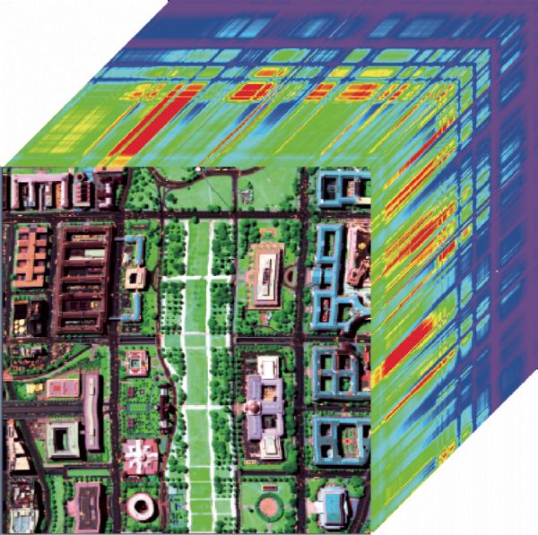
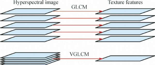
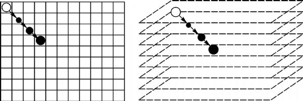
Abstract

A novel approach using volumetric texture and reduced-spectral features is presented for hyperspectral image classification. Using this approach, the volumetric textural features were extracted by volumetric gray-level co-occurrence matrices (VGLCM). The spectral features were extracted by minimum estimated abundance covariance (MEAC) and linear prediction (LP)-based band selection, and a semi-supervised k-means (SKM) clustering method with deleting the worst cluster (SKMd) band-clustering algorithms. Moreover, four feature combination schemes were designed for hyperspectral image classification by using spectral and textural features. It has been proven that the proposed method using VGLCM outperforms the gray-level co-occurrence matrices (GLCM) method, and the experimental results indicate that the combination of spectral information with volumetric textural features leads to an improved classification performance in hyperspectral imagery.

Keywords fusion hyperspectral imagery image classification volumetric textural feature spectral feature

Corresponding Author(s): Peijun DU

Online First Date: 14 November 2014 Issue Date: 30 April 2015

Cite this article:

Hongjun SU,Yehua SHENG,Peijun DU, et al. Hyperspectral image classification based on volumetric texture and dimensionality reduction[J]. Front. Earth Sci., 2015, 9(2): 225-236.

URL:

https://academic.hep.com.cn/fesci/EN/10.1007/s11707-014-0473-4
https://academic.hep.com.cn/fesci/EN/Y2015/V9/I2/225

Fig.1 Hyperspectral image cube for Washington DC Mall data

Fig.2 Texture computation of GLCM and VGLCM

Tab.1 Directions of pairwise pixels for VGLCM

Fig.3 Two-dimensional (2D; left) and three-dimensional (3D; right) semi-variogram analysis for texture extraction

Fig.4 Classification framework for hyperspectral image analysis

Tab.2 Feature fusion schemes for hyperspectral image classification

Tab.3 Training and test samples for DC Mall data

Tab.4 Training and test samples for Indian Pines

Fig.5 Texture samples for different objects

Fig.6 Various box sizes for VGLCM of D.C. Mall dataset. (a) Road I; (b) Road II; (c) Trees I; (d) Trees II; (e) Grass I; (f) Grass II; (g) Building I; (h) Building II

Fig.7 Various window sizes for GLCM of D.C. Mall dataset

Fig.8 Textures extracted using GLCM (left) and VGLCM (right). (a) Variance; (b) Contrast; (c) Dissimilarity; (d) Energy; (e) Entropy; (f) Homogeneity

Fig.9 Classification maps using GLCM and VGLCM textures for D.C. Mall data. (a) 5 selected bands+6 texture features (GLCM); (b) 5 selected bands+6 texture features (VGLCM); (c) 5 clusters+6 texture features (GLCM); (d) 5 clusters+6 texture features (VGLCM)

Tab.5

Tab.6 Classification results for spectral and texture feature fusion

Fig.10 Classification comparison using spectral and texture data

1	Angelo N P, Haertel V (2003). On the application of Gabor filtering in supervised image classification. Int J Remote Sens, 24(10): 2167–2189 https://doi.org/10.1080/01431160210163146
2	Benediktsson J A, Palmason J A, Sveinsson J R (2005). Classification of hyperspectral data from urban areas based on extended morphological profiles. IEEE Trans Geosci Rem Sens, 43(3): 480–491 https://doi.org/10.1109/TGRS.2004.842478
3	Bernabe S, Marpu P R, Plaza A, Mura M D, Benediktsson J A (2014). Spectral-spatial classification of multispectral images using kernel feature space representation. IEEE Geosci Remote Sens Lett, 11(1): 288–292 https://doi.org/10.1109/LGRS.2013.2256336
4	Chang C I (2003). Hyperspectral Imaging: Techniques for Spectral Detection and Classification. New York: Kluwer Academic/Plenum Publishers, 13–15
5	Chang C I (2013). Hyperspectral Data Processing: Algorithm Design and Analysis. New Jersey: Wiley-Interscience, 1–5
6	Chen C, Li W, Tramel E W, Cui M, Prasad S, Fowler J E (2014a). Spectral–spatial preprocessing using multihypothesis prediction for noise-robust hyperspectral image classification. IEEE Journal of Selected Topics in Applied Earth Observations and Remote Sensing, 7(4): 1047–1059 https://doi.org/10.1109/JSTARS.2013.2295610
7	Chen C, Li W, Tramel E W, Fowler J E (2014b). Reconstruction of hyperspectral imagery from random projections using multihypothesis prediction. IEEE Trans Geosci Rem Sens, 52(1): 365–374 https://doi.org/10.1109/TGRS.2013.2240307
8	Gamba P, Dell’ Acqua F, Lisini G, Trianni G (2007). Improved VHR urban area mapping exploiting object boundaries. IEEE Trans Geosci Rem Sens, 45(8): 2676–2682 https://doi.org/10.1109/TGRS.2007.899811
9	Haralick R M, Shanmugam K, Dinstein I H (1973). Texture features for image classification. IEEE Trans Syst Man Cybern, 3(6): 610–621 https://doi.org/10.1109/TSMC.1973.4309314
10	Huang X, Zhang L, Gong W (2011). Information fusion of aerial images and LIDAR data in urban areas: vector stacking, re-classification, and post-processing approaches. Int J Remote Sens, 32(1): 69–84 https://doi.org/10.1080/01431160903439882
11	Jackson Q, Landgrebe D (2002). Adaptive bayesian contextual classification based on markov random fields. IEEE Trans Geosci Rem Sens, 40(11): 2454–2463 https://doi.org/10.1109/TGRS.2002.805087
12	Li J, Bioucas-Dias J, Plaza A (2012). Spectral-spatial hyperspectral image segmentation using subspace multinomial logistic regression and markov random fields. IEEE Trans Geosci Rem Sens, 50(3): 809–823 https://doi.org/10.1109/TGRS.2011.2162649
13	Liu K, Du Q, Yang H, Ma B (2010). Optical flow and principle component analysis-based motion detection in outdoor videos. EURASIP J Adv Signal Process, 2010: 680623 https://doi.org/10.1155/2010/680623
14	Liu K, Ma B, Du Q, Chen G (2012). Fast motion detection from airborne videos using graphics processing units. J Appl Remote Sens, 6(1): 061505
15	Marceau D J, Howarth P J, Dubois J M, Gratton D J (1990). Evaluation of the grey-level co-occurrence matrix method, for land-cover classification using SPOT imagery. IEEE Trans Geosci Rem Sens, 28(4): 513–519 https://doi.org/10.1109/TGRS.1990.572937
16	Mokji M M, Bakar S A R A (2007). Adaptive thresholding based on co-occurrence matrix edge information. Journal of Computers, 2(8): 44–52 https://doi.org/10.4304/jcp.2.8.44-52
17	Mura M D, Villa A, Benediktsson J A, Chanussot J, Bruzzone L (2011). Classification of hyperspectral images by using extended morphological attribute profiles and independent component analysis. IEEE Geosci Remote Sens Lett, 8(3): 541–545
18	Nyoungui A N, Tonye E, Akono A (2002). Evaluation of speckle filtering and texture analysis methods for land cover classification from SAR images. Int J Remote Sens, 23(9): 1895–1925 https://doi.org/10.1080/01431160110036157
19	Plaza J, Plaza A, Barra C (2009). Multi-channel morphological profiles for classification of hyperspectral image data using support vector machines. Sensors (Basel Switzerland), 9(1): 196–218 https://doi.org/10.3390/s90100196
20	Rahman A F, Gamon J A, Sims D A, Schmidts M (2003). Optimum pixel size for hyperspectral studies of ecosystem function in southern California chaparral and grassland. Remote Sens Environ, 84(2): 192–207 https://doi.org/10.1016/S0034-4257(02)00107-4
21	Rajadell O, Garcia-Sevilla P, Pla F (2013). Spectral–spatial pixel characterization using gabor filters for hyperspectral image classification. IEEE Geosci Remote Sens Lett, 10(4): 860–864 https://doi.org/10.1109/LGRS.2012.2226426
22	Su H, Du Q (2012). Hyperspectral band clustering and band selection for urban land cover classification. Geocarto Int, 27(5): 395–411 https://doi.org/10.1080/10106049.2011.643322
23	Su H, Sheng Y, Du P, Liu K (2012). Adaptive affinity propagation with spectral angle mapper for semi-supervised hyperspectral band selection. Appl Opt, 51(14): 2656–2663 https://doi.org/10.1364/AO.51.002656
24	Su H, Yang H, Du Q, Sheng Y (2011). Semi-supervised band clustering for dimensionality reduction of hyperspectral imagery. IEEE Geosci Remote Sens Lett, 8(6): 1135–1139 https://doi.org/10.1109/LGRS.2011.2158185
25	Tsai F, Chang C K, Rau J Y, Lin T H, Liu G R (2007). 3D computation of gray level co-occurrence in hyperspectral image cubes. Lect Notes Comput Sci, 4679: 429–440 https://doi.org/10.1007/978-3-540-74198-5_33
26	Yang H, Du Q, Su H, Sheng Y (2011). An efficient method for supervised hyperspectral band selection. IEEE Geosci Remote Sens Lett, 8(1): 138–142 https://doi.org/10.1109/LGRS.2010.2053516
27	Yang H, Ma B, Du Q, Yang C (2010). Improving urban land use and land cover classification from high-spatial-resolution hyperspectral imagery using contextual information. J Appl Remote Sens, 4(1): 041890 https://doi.org/10.1117/1.3491192

[1]	Tianjie LEI, Jie FENG, Cuiying ZHENG, Shuguang LI, Yang WANG, Zhitao WU, Jingxuan LU, Guangyuan KAN, Changliang SHAO, Jinsheng JIA, Hui CHENG. Review of drought impacts on carbon cycling in grassland ecosystems[J]. Front. Earth Sci., 2020, 14(2): 462-478.
[2]	Zheng WANG, Zhihua MAO, Junshi XIA, Peijun DU, Liangliang SHI, Haiqing HUANG, Tianyu WANG, Fang GONG, Qiankun ZHU. Data fusion in data scarce areas using a back-propagation artificial neural network model: a case study of the South China Sea[J]. Front. Earth Sci., 2018, 12(2): 280-298.
[3]	Hongjun SU, Shufang TIAN, Yue CAI, Yehua SHENG, Chen CHEN, Maryam NAJAFIAN. Optimized extreme learning machine for urban land cover classification using hyperspectral imagery[J]. Front. Earth Sci., 2017, 11(4): 765-773.
[4]	Sizhang TANG,Chaomin SHEN,Guixu ZHANG. Adaptive regularized scheme for remote sensing image fusion[J]. Front. Earth Sci., 2016, 10(2): 236-244.
[5]	Shaolei TANG,Xiaofeng YANG,Di DONG,Ziwei LI. Merging daily sea surface temperature data from multiple satellites using a Bayesian maximum entropy method[J]. Front. Earth Sci., 2015, 9(4): 722-731.
[6]	Wei WANG,Xinfeng YAO,Minhe JI,Jiao ZHANG. Spectral data treatments for impervious endmember derivation and fraction mapping from Landsat ETM+ imagery: a comparative analysis[J]. Front. Earth Sci., 2015, 9(2): 179-191.
[7]	Zhan TIAN, Honglin ZHONG, Runhe SHI, Laixiang SUN, Günther FISCHER, Zhuoran LIANG. Estimating potential yield of wheat production in China based on cross-scale data-model fusion[J]. Front Earth Sci, 2012, 6(4): 364-372.

Viewed

Full text

Abstract

Cited

Shared

Discussed