Quantifying the early snowmelt event of 2015 in the Cascade Mountains, USA by developing and validating MODIS-based snowmelt timing maps

doi:10.1007/s11707-018-0719-7

Front. Earth Sci.

2018, Vol. 12

Issue (4) : 693-710 https://doi.org/10.1007/s11707-018-0719-7

RESEARCH ARTICLE

Quantifying the early snowmelt event of 2015 in the Cascade Mountains, USA by developing and validating MODIS-based snowmelt timing maps

Donal O’Leary III^1,²(

), Dorothy Hall^3,⁴, Michael Medler², Aquila Flower²

¹. University of Maryland, Department of Geographical Sciences, College Park, MD 20740, USA
². Western Washington University, Department of Environmental Studies, Bellingham, WA 98225, USA
³. National Aeronautics and Space Administration, Goddard Space Flight Center, Greenbelt, MD 20771, USA
⁴. Earth System Science Interdisciplinary Center, University of Maryland, College Park, MD 20740, USA

Download: PDF(14864 KB) HTML
Export: BibTeX | EndNote | Reference Manager | ProCite | RefWorks

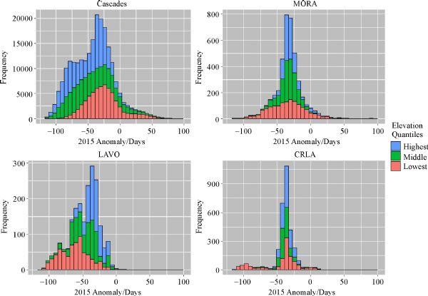
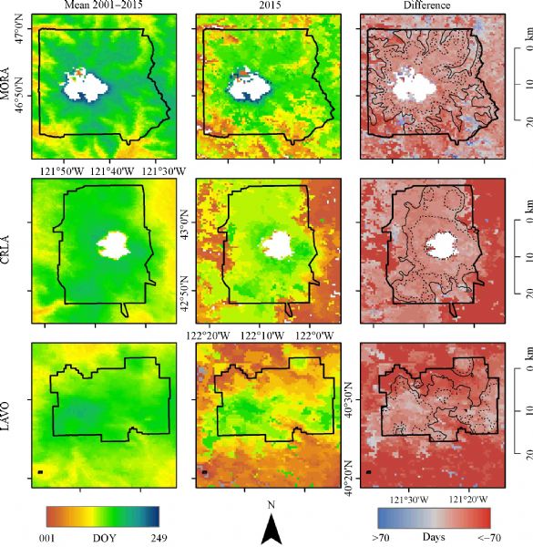
Abstract

Spring snowmelt serves as the major hydrological contribution to many watersheds of the US West. Since the 1970s the conterminous western USA has seen an earlier arrival of spring snowmelt. The extremely low snowpack and early melt of 2015 in the Cascade Mountains may be a harbinger of winters to come, underscoring the interest in advancements in spring snowmelt monitoring. Target-of-opportunity and point measurements of snowmelt using meteorological stations or stream gauges are common sources of these data, however, there have been few attempts to identify snowmelt timing using remote sensing. In this study, we describe the creation of snowmelt timing maps (STMs) which identify the day of year that each pixel of a remotely sensed image transitions from “snow-covered” to “no snow” during the spring melt season, controlling for cloud coverage and ephemeral spring snow storms. Derived from the 500 m MODerate-resolution Imaging Spectroradiometer (MODIS) standard snow map, MOD10A2, this new dataset provides annual maps of snowmelt timing, with corresponding maps of cloud interference and interannual variability in snow coverage from 2001–2015. We first show that the STMs agree strongly with in-situ snow telemetry (SNOTEL) meteorological station measurements in terms of snowmelt timing. We then use the STMs to investigate the early snowmelt event of 2015 in the Cascade Mountains, USA, highlighting the protected areas of Mt. Rainier, Crater Lake, and Lassen Volcanic National Parks. In 2015 the Cascade Mountains experienced snowmelt 41 days earlier than the 2001–2015 average, with 25% of its land area melting>65 days earlier than average. The upper elevations of the Cascade Mountains experienced the greatest snowmelt anomaly. Our results are relevant to land managers and biologists as they plan adaptation strategies for mitigating the effects of climate change throughout temperate mountains.

Keywords Cascade Mountains snowmelt spring phenology MODIS remote sensing

Corresponding Author(s): Donal O’Leary III

Just Accepted Date: 21 June 2018 Online First Date: 03 August 2018 Issue Date: 20 November 2018

Cite this article:

Donal O’Leary III,Dorothy Hall,Michael Medler, et al. Quantifying the early snowmelt event of 2015 in the Cascade Mountains, USA by developing and validating MODIS-based snowmelt timing maps[J]. Front. Earth Sci., 2018, 12(4): 693-710.

URL:

https://academic.hep.com.cn/fesci/EN/10.1007/s11707-018-0719-7
https://academic.hep.com.cn/fesci/EN/Y2018/V12/I4/693

Fig.1 Overview of study area elevation including Washington, Oregon, and California state boundaries (thick grey lines), the Cascade Mountains Ecoregion, and park unit polygons (thick black lines, left), and close-up views of Mt. Rainier (MORA), Crater Lake (CRLA) (with thin line of Cascade Mountains boundary visible crossing SE corner of the park), and Lassen Volcanic (LAVO) National Parks (right). SNOTEL stations are indicated by white circles with black outlines. Note that water bodies (including Crater Lake itself) are not differentiated on the elevation surface. Elevation data (30 m) resampled to resolution and registration of the STM data (500 m).

Tab.1 Explanation of snowmelt and cloud interference logic for each pixel. Case describes the series of consecutive MOD10A2 image values. Snowmelt DOY is the resulting value in the STM. All DOY values are relative to the DOY of the no-snow MODIS image. Cloud interference values represent the number of temporally-interpolated images+1, to avoid values of zero which may be confused as ‘No Data’ values in the STM dataset. For example, case 5 (bottom) shows a snow-covered composite image and a snow-free composite image separated by 4 consecutive images of no-snow. The resulting snowmelt value is interpolated to be the DOY of the snow-free image minus 16 (i.e., 32 days of separation between the snow- and no-snow images, divided by two), with a cloud interference value of 5 (4 cloud images, plus 1)

Tab.2 Pixel population sizes and elevation quantile limits for areas of interest (Q1= lowest elevation, Q3= highest)

Fig.2 Overview of STMs for the Cascade Mountains including outline of the Cascade Mountains Ecoregion (thick black line) and state boundaries (grey lines). Mean STM from 2001–2015, 2015 alone, and 2015-Mean difference are shown from left to right. White regions indicate areas with Count values less than 8 (mean) or no snow snowmelt detected (2015). Elevation quantile contour lines are omitted for clarity.

Fig.3 2015 snowmelt anomaly distributions by study area (plot) and elevation quantile (color). Count describes the number of pixels with side length of ~500 meters. See Tables 2 and 3 for detailed statistics. Note how the Cascade Mountains as a whole experienced greater anomalies in the highest quantile (blue), while Mt. Rainier (MORA), Crater Lake (CRLA), and Lassen Volcanic (LAVO) National Parks experienced a greater anomaly in the lowest quantile (red).

Fig.4 Maps of Mt. Rainier (MORA), Crater Lake (CRLA), and Lassen Volcanic (LAVO) National Parks (top to bottom), showing 2001?2015 mean STM, 2015 STM, and 2015-mean difference (left to right). In the difference panels, the thin solid black line indicates the lower bound of the middle elevation quantile, and the dashed line indicates the lower bound of the upper elevation quantile (Table 2). The year 2015 shows early snowmelt for most of each park, however the lower-elevation areas surrounding the volcanoes show a greater difference than the high-elevation areas within the parks. White regions indicate areas with Count values less than 8 (mean) or no snow snowmelt detected for the year 2015, primarily located in the glaciers of MORA, and Crater Lake itself.

Tab.3 Descriptive statistics for distributions of anomalies by study area and elevation quantile (Q1= lowest elevation, Q3= highest). Mean snowmelt timing includes years 2001?2015 and excludes points with fewer than 8 years of coverage. 2015 anomaly is calculated on a per-pixel basis by subtracting the mean from the year 2015

Tab.4 Snowmelt timing quantiles for the Cascade Mountains and Mount Rainier, Crater Lake, and Lassen Volcanic National Parks. The values shown here describe 2015 snowmelt timing anomaly experienced by a given percentage of land area for each study area in days. For example, 10% of the land area for the Cascade Mountains had a snowmelt timing anomaly of ≥83.73 days earlier than the 2001?2015 average

Fig.5 Cloud Interference and Count maps for the Cascade Mountains and national parks of interest. Mean cloud cover maps show the mean cloud interference values per pixel from 2001?2015, as described in Table 1. Count maps show the number of years of STM coverage, with mountainous regions experiencing accumulation and observable snowmelt for most, if not all, of the 15 years on record (darkest blue, ‘Count’ images). Note that mean cloud interference values disregard null values (years without STM values) and may therefore overestimate mean cloud interference for regions with low Count values. White areas (MORA glaciers, Crater Lake itself, Northern California valleys) have no snow observations for the period of record.

Fig.6 Snow-cover depletion curves (SCDCs) for the Cascade Mountains, MORA, CRLA, and LAVO. Mean SCDC is calculated as the mean (black) of all SCDCs from 2001?2015, not from the mean STM image. The year 2015 (red) is clearly the earliest melt of all years for all regions, with an earlier initial melt and earlier complete melt than all other years. Note that each X-axis is focused on melt season for each region.

Table A1 Examples of the differences in the STM and SNODOY results. In ideal, clear sky conditions the STM reports snowmelt within 8-day ranges (001, 009, 017, 025, etc.), whereas the SNOTEL stations allow for a daily time step

Fig. A1 Histograms illustrating the errors between the Snowmelt Timing Maps (STMs) and SNOTEL stations (days, x axis; frequency, y-axis). Errors are calculated by subtracting the SNOTEL melt Day Of Year (SNODOY) from the STM DOY. Errors are non-normally distributed (α = 0.10) about means ranging from 0.81 (2008) to 7.40 (2015), except for 2004, which is normally distributed.

Fig. A2 Histograms describing the errors between the Snowmelt Timing Maps (STMs) and SNOTEL stations (days, x axis; frequency, y-axis) for all SNOTEL locations within the Cascade Mountains Ecoregion for years 2001?2015. Years marked with an asterisk are normally distributed (α = 0.10). Means range from 17.05 (2008) to+5.03 (2001).

Fig. A3 Histograms of errors between the Snowmelt Timing Maps (STMs) and SNOTEL stations (days, x axis; frequency, y-axis) for the entire period of record for all SNOTEL sites, and those within the Cascade Mountains Ecoregion, calculated as STM-SNODOY+3.5. Colors indicate cloud interference value (1= no cloud interference, 5= four consecutive 8-day composite images of clouds). Both populations are centered about means of 4.31 and ?4.76 with standard deviations of 17.53 and 21.70, respectively. Clouds interfered with 10.67% of readings for all SNOTEL stations, and 11.92% of those within the Cascade Mountains Ecoregion.

Table A2 Description of the population of validation errors by cloud interference value

1	J T Abatzoglou, C A Kolden (2013). Relationships between climate and macroscale area burned in the western United States. Int J Wildland Fire, 22(7): 1003–1020 https://doi.org/10.1071/WF13019
2	A Barrett (2003). National Operational Hydrologic Remote Sensing Center SNOw Data Assimilation System (SNODAS) Products at National Snow and Ice Data Center. Special Report #11
3	W D Billings, L C Bliss (1959). An alpine snowbank environment and its effects on vegetation, plant development, and productivity. Ecology, 40(3): 388–397 https://doi.org/10.2307/1929755
4	R D Brown, B Brasnett, D Robinson (2003). Gridded North American monthly snow depth and snow water equivalent for GCM evaluation. Atmos-ocean, 41(1): 1–14 https://doi.org/10.3137/ao.410101
5	K L Brubaker, R T Pinker, E Deviatova (2005). Evaluation and comparison of MODIS and IMS snow-cover estimates for the continental United States using station data. J Hydrometeorol, 6(6): 1002–1017 https://doi.org/10.1175/JHM447.1
6	C Cornelius, A Leingärtner, B Hoiss, J Krauss, I Steffan-Dewenter, A Menzel (2013). Phenological response of grassland species to manipulative snowmelt and drought along an altitudinal gradient. J Exp Bot, 64(1): 241–251 https://doi.org/10.1093/jxb/ers321
7	C J Crawford (2014). MODIS Terra Collection 6 fractional snow cover validation in mountainous terrain during spring snowmelt using Landsat TM and ETM+. Hydrol Processes, 29(1): 128–138 https://doi.org/10.1002/hyp.10134
8	S E Dickerson-Lange, R F Gersonde, J A Hubbart, T E Link, A W Nolin, G H Perry, T R Roth, N E Wayand, J D Lundquist (2017). Snow disappearance timing is dominated by forest effects on snow accumulation in warm winter climates of the Pacific Northwest, United States. Hydrol Processes, 31(10): 1846–1862 https://doi.org/10.1002/hyp.11144
9	S R Fassnacht, G A Sexstone, A H Kashipazha, J I López-Moreno, M F Jasinski, S K Kampf, B C Von Thaden (2016). Deriving snow-cover depletion curves for different spatial scales from remote sensing and snow telemetry data. Hydrol Processes, 30(11): 1708–1717 https://doi.org/10.1002/hyp.10730
10	S Ganguly, M A Friedl, B Tan, X Zhang, M Verma (2010). Land surface phenology from MODIS: characterization of the Collection 5 global land cover dynamics product. Remote Sens Environ, 114(8): 1805–1816 https://doi.org/10.1016/j.rse.2010.04.005
11	K E Gleason, A W Nolin, T R Roth (2017). Developing a representative snow-monitoring network in a forested mountain watershed. Hydrol Earth Syst Sci, 21(2): 1137–1147 https://doi.org/10.5194/hess-21-1137-2017
12	D K Hall, C J Crawford, N E DiGirolamo, G A Riggs, J L Foster (2015). Detection of earlier snowmelt in the Wind River Range, Wyoming, using Landsat imagery, 1972–2013. Remote Sens Environ, 162(1): 45–54 https://doi.org/10.1016/j.rse.2015.01.032
13	D K Hall, J L Foster, N E, DiGirolamo G A Riggs (2012). Snow cover, snowmelt timing, and stream power in the Wind River Range, Wyoming. Geomorphology, 137(1): 87–93 https://doi.org/10.1016/j.geomorph.2010.11.011
14	D K Hall, G A Riggs (2007). Accuracy assessment of the MODIS snow products. Hydrol Processes, 21(12): 1534–1547 https://doi.org/10.1002/hyp.6715
15	D K Hall, G A Riggs (2016). MODIS/Terra Snow Cover Daily L3 Global 500 m Grid, Version 6. NASA National Snow and Ice Data Center Distributed Active Archive Cente https://doi.org/10.5067/MODIS/MOD10A1.006
16	D K Hall, V V Salomonson, G A Riggs (2006). MODIS/Terra Snow Cover 8-Day L3 Global 500m Grid. Version 5. National Snow and Ice Data Center
17	J W Homan, C H Luce, J P McNamara, N F Glenn (2011). Improvement of distributed snowmelt energy balance modeling with MODIS-based NDSI-derived fractional snow-covered area data. Hydrol Processes, 25(4): 650–660 https://doi.org/10.1002/hyp.7857
18	D W Inouye (2008). Effects of climate change on phenology, frost damage, and floral abundance of Montane Wildflowers. Ecology, 89(2): 353–362 https://doi.org/10.1890/06-2128.1
19	D W Inouye, M A Morales, G J Dodge (2002). Variation in timing and abundance of flowering by Delphinium barbeyi Huth (Ranunculaceae): the roles of snowpack, frost, and La Niña, in the context of climate change. Oecologia, 130(4): 543–550 https://doi.org/10.1007/s00442-001-0835-y
20	J P Iorio, P B Duffy, B Govindasamy, S L Thompson, M Khairoutdinov, D Randall (2004). Effects of model resolution and subgrid-scale physics on the simulation of precipitation in the continental United States. Clim Dyn, 23(3–4): 243–258 https://doi.org/10.1007/s00382-004-0440-y
21	P Jönsson, L Eklundh (2004). TIMESAT‒ a program for analysing time-series of satellite sensor data. Comput Geosci, 30(8): 833–845 https://doi.org/10.1016/j.cageo.2004.05.006
22	A G Klein, A C Barnett (2003). Validation of daily MODIS snow cover maps of the Upper Rio Grande River Basin for the 2000–2001 snow year. Remote Sens Environ, 86(2): 162–176 https://doi.org/10.1016/S0034-4257(03)00097-X
23	J S Littell, D McKenzie, D L Peterson, A L Westerling (2009). Climate and wildfire area burned in western U.S. ecoprovinces, 1916—2003. Ecol Appl, 19(4): 1003–1021 https://doi.org/10.1890/07-1183.1
24	J D Lundquist, S E Dickerson-Lange, J A Lutz, N C Cristea (2013). Lower forest density enhances snow retention in regions with warmer winters: a global framework developed from plot-scale observations and modeling. Water Resour Res, 49(10): 6356–6370 https://doi.org/10.1002/wrcr.20504
25	S A Margulis, G Cortés, M Girotto, M Durand (2016b). A Landsat-Era Sierra Nevada snow reanalysis (1985–2015). J Hydrometeorol, 17(4): 1203–1221 https://doi.org/10.1175/JHM-D-15-0177.1
26	SA Margulis, G Cortés, M Girotto, LS Huning, D Li, M Durand (2016a). Characterizing the extreme 2015 snowpack deficit in the Sierra Nevada (USA) and the implications for drought recovery. Geophysical Research Letters, 43(12): 2016GL068520. DOI:10.1002/2016GL068520
27	G J McCabe, M P Clark, L E Hay (2007). Rain-on-snow events in the western United States. Bull Am Meteorol Soc, 88(3): 319–328 https://doi.org/10.1175/BAMS-88-3-319
28	C Moore, S Kampf, B Stone, E Richer (2015). A GIS-based method for defining snow zones: application to the western United States. Geocarto Int, 30(1): 62–81 https://doi.org/10.1080/10106049.2014.885089
29	P W Mote, A F Hamlet, M P Clark, D P Lettenmaier (2005). Declining mountain snowpack in western North America. Bull Am Meteorol Soc, 86(1): 39–49 https://doi.org/10.1175/BAMS-86-1-39
30	K N Musselman, N P Molotch, S A Margulis (2017). Snowmelt response to simulated warming across a large elevation gradient, southern Sierra Nevada, California. Cryosphere, 11(6): 2847–2866 https://doi.org/10.5194/tc-11-2847-2017
31	R Narasimhan, D Stow (2010). Daily MODIS products for analyzing early season vegetation dynamics across the North Slope of Alaska. Remote Sens Environ, 114(6): 1251–1262 https://doi.org/10.1016/j.rse.2010.01.017
32	A W Nolin, C Daly (2006). Mapping “At Risk” Snow in the Pacific Northwest. J Hydrometeorol, 7(5): 1164–1171 https://doi.org/10.1175/JHM543.1
33	A W Nolin, E A Sproles, R L Crumley, A Wilson, E Mar, M van de Kerk, L Prugh (2017). Cloud-based Computing and Applications of New Snow Metrics for Societal Benefit. AGU Fall Meeting Abstracts, 22
34	NPS (2016a). Science and Learning Center.
35	NPS (2016b). Ongoing and Past Research.
36	NPS (2016c). Klamath Network Inventory and Monitoring.
37	NRCS (2016). NRCS National Water and Climate Center \| SNOTEL Data & Products.
38	D S O’Leary III , T D Bloom, J C Smith, C R Zempf, M J Medler (2016). A new method comparing snowmelt timing with annual area burned. Fire Ecol, 12(1): 41–51 https://doi.org/10.4996/fireecology.1201041
39	D S O’Leary III , D K Hall, M J Medler, R A Matthews, A Flower (2017). Snowmelt Timing Maps Derived from MODIS for North America, 2001‒2015. Oak Ridge National Laboratory.
40	D S O’Leary III , J L Kellermann, C Wayne (2018). Snowmelt timing, phenology, and growing season length in conifer forests of Crater Lake National Park, USA. Int J Biometeorol, 62(2): 273–285 https://doi.org/10.1007/s00484-017-1449-3
41	B H Ramsay (1998). The interactive multisensor snow and ice mapping system. Hydrol Processes, 12(10–11): 1537–1546 https://doi.org/10.1002/(SICI)1099-1085(199808/09)12:10/11<1537::AID-HYP679>3.0.CO;2-A
42	I Rangwala, J R Miller (2012). Climate change in mountains: a review of elevation-dependent warming and its possible causes. Clim Change, 114(3–4): 527–547 https://doi.org/10.1007/s10584-012-0419-3
43	G A Riggs, D K Hall, M O Román (2017). Overview of NASA’s MODIS and visible infrared imaging radiometer suite (VIIRS) snow-cover earth system data records. Earth Syst Sci Data, 9(2): 765–777 https://doi.org/10.5194/essd-9-765-2017
44	T R Roth, A W Nolin (2017). Forest impacts on snow accumulation and ablation across an elevation gradient in a temperate montane environment. Hydrol Earth Syst Sci, 21(11): 5427–5442 https://doi.org/10.5194/hess-21-5427-2017
45	K A Semmens, J Ramage (2012). Investigating correlations between snowmelt and forest fires in a high latitude snowmelt dominated drainage basin. Hydrol Processes, 26(17): 2608–2617 https://doi.org/10.1002/hyp.9327
46	J A Sherwood, D M Debinski, P C Caragea, M J Germino (2017). Effects of experimentally reduced snowpack and passive warming on montane meadow plant phenology and floral resources. Ecosphere, 8(3): e01745 https://doi.org/10.1002/ecs2.1745
47	A Simic, R Fernandes, R Brown, P Romanov, W Park (2004). Validation of VEGETATION, MODIS, and GOES+ SSM/I snow-cover products over Canada based on surface snow depth observations. Hydrol Processes, 18(6): 1089–1104 https://doi.org/10.1002/hyp.5509
48	E A Sproles, A W Nolin, K Rittger, T H Painter (2013). Climate change impacts on maritime mountain snowpack in the Oregon Cascades. Hydrol Earth Syst Sci, 17(7): 2581–2597 https://doi.org/10.5194/hess-17-2581-2013
49	E A Sproles, T R Roth, A W Nolin (2017). A spatial-probabilistic assessment of the extraordinarily low snowpacks of 2014 and 2015 in the Oregon Cascades. Cryosphere, 11(1): 331–341 https://doi.org/10.5194/tc-11-331-2017
50	H Steltzer, C Landry, T H Painter, J Anderson, E Ayres (2009). Biological consequences of earlier snowmelt from desert dust deposition in alpine landscapes. Proc Natl Acad Sci USA, 106(28): 11629–11634 https://doi.org/10.1073/pnas.0900758106
51	I T Stewart (2009). Changes in snowpack and snowmelt runoff for key mountain regions. Hydrol Processes, 23(1): 78–94 https://doi.org/10.1002/hyp.7128
52	S C Swenson, D M Lawrence (2012). A new fractional snow-covered area parameterization for the Community Land Model and its effect on the surface energy balance. J Geophys Res D Atmospheres, 117(D21): D21107 https://doi.org/10.1029/2012JD018178
53	A A Tahir, P Chevallier, Y Arnaud, B Ahmad (2011). Snow cover dynamics and hydrological regime of the Hunza River basin, Karakoram Range, Northern Pakistan. Hydrol Earth Syst Sci, 15(7): 2275–2290 https://doi.org/10.5194/hess-15-2275-2011
54	Ø Totland, J M Alatalo (2002). Effects of temperature and date of snowmelt on growth, reproduction, and flowering phenology in the arctic/alpine herb, Ranunculus glacialis. Oecologia, 133(2): 168–175 https://doi.org/10.1007/s00442-002-1028-z
55	University of Wyoming (2017). Grand Teton National Park Service Research Needs 2017.
56	USGS (2014). Geologic Provinces of the United States: Pacific.
57	USGS (2017). National Elevation Dataset (NED) The Long Term Archive.
58	USGS (2018). United States Geological Survey Current Water Data for the Nation.
59	USGSA (2017). Data.gov US General Services Administration. In: Data.gov.
60	A L Westerling, H G Hidalgo, D R Cayan, T W Swetnam (2006). Warming and earlier spring increase western U.S. forest wildfire activity. Science, 313(5789): 940–943 https://doi.org/10.1126/science.1128834
61	AL Westerling (2016). Increasing western US forest wildfire activity: sensitivity to changes in the timing of spring. Philosophical Transactions of the Royal Society B: Biological Sciences, 371(1696): 1–10. DOI:10.1098/rstb.2015.0178
62	A Wolf, N B Zimmerman, W R L Anderegg, P E Busby, J Christensen (2016). Altitudinal shifts of the native and introduced flora of California in the context of 20th-century warming. Glob Ecol Biogeogr, 25(4): 418–429 https://doi.org/10.1111/geb.12423
63	S Yu, P V Bhave, R L Dennis, R Mathur (2007). Seasonal and regional variations of primary and secondary organic aerosols over the continental United States: semi-empirical estimates and model evaluation. Environ Sci Technol, 41(13): 4690–4697 https://doi.org/10.1021/es061535g
64	X Zhang, M A Friedl, C B Schaaf (2006). Global vegetation phenology from moderate resolution imaging spectroradiometer (MODIS): evaluation of global patterns and comparison with in situ measurements. J Geophys Res Biogeosci, 111(G4): G04017 doi:10.1029/2006JG000217

[1]	Munkhdulam OTGONBAYAR, Clement ATZBERGER, Erdenesukh SUMIYA, Sainbayar DALANTAI, Jonathan CHAMBERS. Estimation of bioclimatic variables of Mongolia derived from remote sensing data[J]. Front. Earth Sci., 2022, 16(2): 323-339.
[2]	Sijun ZHENG, Chen MENG, Jianhui XUE, Yongbo WU, Jing LIANG, Liang XIN, Lang ZHANG. UAV-based spatial pattern of three-dimensional green volume and its influencing factors in Lingang New City in Shanghai, China[J]. Front. Earth Sci., 2021, 15(3): 543-552.
[3]	Herrieth MACHIWA, Bo TIAN, Dhritiraj SENGUPTA, Qian CHEN, Michael MEADOWS, Yunxuan ZHOU. Vegetation dynamics in response to human and climatic factors in the Tanzanian Coast[J]. Front. Earth Sci., 2021, 15(3): 595-605.
[4]	Conghui LI, Lili LIN, Zhenbang HAO, Christopher J. POST, Zhanghao CHEN, Jian LIU, Kunyong YU. Developing a USLE cover and management factor (C) for forested regions of southern China[J]. Front. Earth Sci., 2020, 14(3): 660-672.
[5]	Emre ÇOLAK, Filiz SUNAR. Spatial pattern analysis of post-fire damages in the Menderes District of Turkey[J]. Front. Earth Sci., 2020, 14(2): 446-461.
[6]	Xia LEI, Jiayi PAN, Adam DEVLIN. An ultraviolet to visible scheme to estimate chromophoric dissolved organic matter absorption in a Case-2 water from remote sensing reflectance[J]. Front. Earth Sci., 2020, 14(2): 384-400.
[7]	Jianhong LIU, Clement ATZBERGER, Xin HUANG, Kejian SHEN, Yongmei LIU, Lei WANG. *Modeling grass yields in Qinghai Province, China, based on MODIS NDVI* data—an empirical comparison**[J]. Front. Earth Sci., 2020, 14(2): 413-429.
[8]	Tong LI, Huadong GUO, Li ZHANG, Chenwei NIE, Jingjuan LIAO, Guang LIU. Simulation of Moon-based Earth observation optical image processing methods for global change study[J]. Front. Earth Sci., 2020, 14(1): 236-250.
[9]	Kaiguo FAN, Huaguo ZHANG, Jianjun LIANG, Peng CHEN, Bojian XU, Ming ZHANG. Analysis of ship wake features and extraction of ship motion parameters from SAR images in the Yellow Sea[J]. Front. Earth Sci., 2019, 13(3): 588-595.
[10]	Ying XIONG, Fen PENG, Bin ZOU. Spatiotemporal influences of land use/cover changes on the heat island effect in rapid urbanization area[J]. Front. Earth Sci., 2019, 13(3): 614-627.
[11]	Shichao CUI, Kefa ZHOU, Rufu DING, Guo JIANG. Estimation of copper concentration of rocks using hyperspectral technology[J]. Front. Earth Sci., 2019, 13(3): 563-574.
[12]	Yongfeng WANG, Zhaohui XUE, Jun CHEN, Guangzhou CHEN. Spatio-temporal analysis of phenology in Yangtze River Delta based on MODIS NDVI time series from 2001 to 2015[J]. Front. Earth Sci., 2019, 13(1): 92-110.
[13]	Jianhong LIU, Le LI, Xin HUANG, Yongmei LIU, Tongsheng LI. Mapping paddy rice in Jiangsu Province, China, based on phenological parameters and a decision tree model[J]. Front. Earth Sci., 2019, 13(1): 111-123.
[14]	Igor Appel. Uncertainty in satellite remote sensing of snow fraction for water resources management[J]. Front. Earth Sci., 2018, 12(4): 711-727.
[15]	Xiaojuan HUANG, Mingguo MA, Xufeng WANG, Xuguang TANG, Hong YANG. The uncertainty analysis of the MODIS GPP product in global maize croplands[J]. Front. Earth Sci., 2018, 12(4): 739-749.

Viewed

Full text

Abstract

Cited

Shared

Discussed